Project 2 - Rankine cycle Simulator
Aim:- Create a Rankine Cycle Simulator using MATLAB.
Objective:-
- Calculate the state points of the Rankine Cycle (any type of your choice) based on user inputs.
- Plot the corresponding T-s and h-s plots for the given set of inputs.
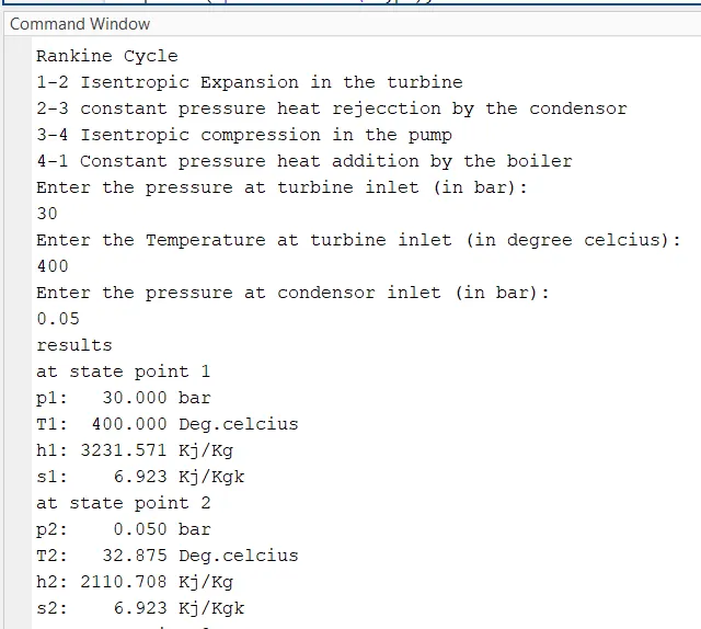
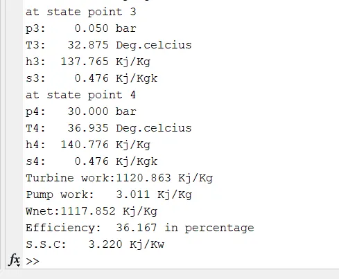
- To get output in Command Window for all state points.
Theory:-
Rankine Cycle:
Rankine Cycle is the Thermodynamic Cycle which describes processes like Heat engine, steam Turbine and Steam Engine, it will extract mechanical energy from some heat source and gives some Useful Work. In Steam Turbine The Rankine cycle principle is used.
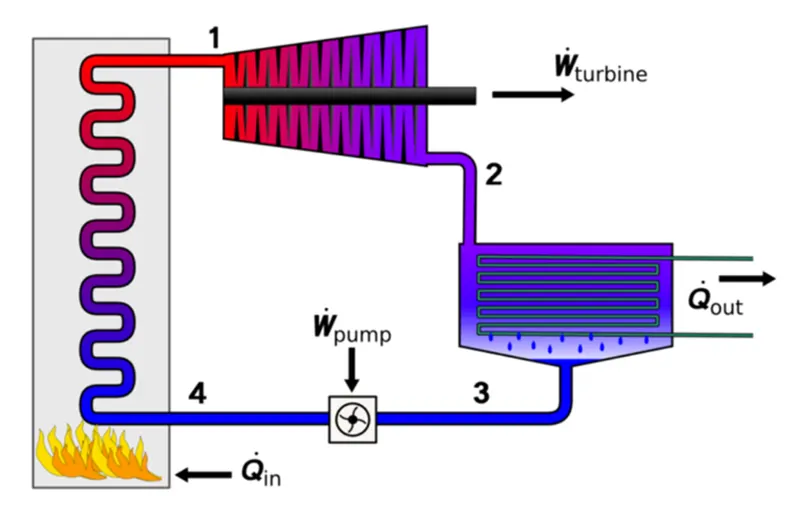
Fig. Rankine Cycle:- Steam Turbine
In Above Fig. we can see that Steam Turbine Working on Rankine Cycle.
Componenets of Steam Turbine
- Turbine
- Condensor
- Pump
- Boiler
Working :
In steam Turbine liquid(mostly Water) is used for Boiling in Boiler, Boiler boils water (Qin) untill it gets converted in to Steam, here heat addition will be done, in that time Pressure will be constant, then this water convert in to high pressure Steam. this steam is supplied to Turbine while this process Pressure will be vary. that steam is used to convert this energy to mechanical energy(Wt). then after Turbine rotates steam will sent to condensor for make Vapour to water(Qout) here heat rejection will be done. then it will be converted in to water then water again sent to Pump for increase the Pressure here Pump required some energy (Wp).
Process:
There are Four Processes in Rankine Cycle:
1) Process 1-2 :Isentropic Expansion in Turbine
Dry Saturated Vapour expand in Turbine, generate power. The shaft is connected to generator ,this results in production of electricity means Conversion of Mechanical energy to Electrical energy.
2) Process 2-3 : Constant Pressure Heat Rejection in Condensor
The expanded vapour passed through Condensor, where it gets condensed and convert in to Liquid again. this liquid again pumped to boiler.
3) Process 3-4 : Isentropic Compression by Pump
In this process water comess into Pump in saturated state then liquid compressed isentropically untill get boiler pressure.
4) Process 4-1 : Constant Pressure Heat Addition in Boiler
In this process water enters into Boiler it converts in to high pressure steam in this process pressure will be constant. in which Liquid phase changed in to Vapour.
Required Inputs:
Turbine Inlet temperature = 400° C
Turbine Inlet Pressure = 30 bars
Turbine Outlet Pressure = 0.05 bars = Condenser Inlet Pressure
Following Formulaes used :
`QIn=h1-h4`
`Wt=h1-h2`
`Qout=h2-h3`
`Wp=h4-h3`
`S.S.C=3600/(Wn)`
Where,
Wn= Net Work
`Thermal Efficiency=(WNet)/(QIn)*100`
MATLAB CODE:
clear all

close all

clc


% print process Description

fprintf('Rankine Cycle\n')

fprintf('1-2 Isentropic Expansion in the turbine\n');

fprintf('2-3 constant pressure heat rejecction by the condensor\n');

fprintf('3-4 Isentropic compression in the pump\n');

fprintf('4-1 Constant pressure heat addition by the boiler\n');


% Inputes

p1=input('Enter the pressure at turbine inlet (in bar):\n');

T1=input('Enter the Temperature at turbine inlet (in degree celcius):\n');

p2=input('Enter the pressure at condensor inlet (in bar):\n');


% calculate state point values

% state-1

h1=XSteam('h_pT',p1,T1);    % Enthalpy at pressure and Temperature 1

s1=XSteam('s_pT',p1,T1);    % Entropy at pressure and Temperature 1


%state-2

s2=s1;                      % s2=s1 because isentropic expansion

sf2=XSteam('sL_p',p2);      % saturated liquid entropy at pressure 2

sg2=XSteam('sV_p',p2);      % saturated Vapour entropy at pressure 2

x2=(s2-sf2)/(sg2-sf2);      % Dryness fraction at state point 2

hf2=XSteam('hL_p',p2);      % saturated liquid enthalpy at pressure 2

hg2=XSteam('hV_p',p2);      % saturated Vapour enthalpy at pressure 2

h2=hf2+(x2*(hg2-hf2));      % Enthalpy at state point 2


%state-3

p3=p2;                      % constant Pressure at Heat Removal process

s3=XSteam('sL_p',p3);       % saturated liquid entropy at pressure 3

h3=XSteam('hL_p',p3);       % saturated liquid enthalpy at pressure 3


%state-4

s4=s3;                      % Isentropic Compression Process

p4=p1;                      % constant pressure heat rejection.


% work done by Turbine

Wt=h1-h2;


% work done to run pump

v3=XSteam('vL_p',p3);

Wp=v3*(p4-p3)*100;

h4=h3+Wp;


% net work

Wnet=Wt-Wp;


% heat in to the System

Qin=h1-h4;


% heat out  to system

Qout=h2-h3;


% Thermal Effficiency

eff=(Wnet/Qin)*100;


% Specific steam consumption

%SSC= mass flow rate per Power

SSC=(3600/Wnet);


% calculating Temperatures at state points 2,3,4

T3=XSteam('Tsat_p',p3);

T2=T3;

cp4=XSteam('cp_ps',p4,s4);

cv4=XSteam('cv_ps',p4,s4);

k=cp4/cv4;

T4=T3/((p3/p4)^((k-1)/k));


% calculating Temperature, enthalpy,entropy at Saturated vapour and liquid


T6=XSteam('Tsat_p',p1);

s5=XSteam('sL_p',p1);

s6=XSteam('sV_p',p1);

h5=XSteam('hL_p',p1);

h6=XSteam('hV_p',p1);

T5=T6;


% plotting the saturation Curve

T=linspace(1,375,1000);

for i=1:length(T)

    sf(i)=XSteam('sL_T',T(i));

    sg(i)=XSteam('sV_T',T(i));

    hf(i)=XSteam('hL_T',T(i));

    hg(i)=XSteam('hV_T',T(i));

end


% plotting the T-S diagram

figure(1)

hold on

plot(sf,T,'color','r','linewidth',1)

plot(sg,T,'color','r','linewidth',1)

plot([s1 s2],[T1 T2], 'K','LineWidth',2)

plot([s2 s3],[T2 T3], 'K','LineWidth',2)

plot([s3 s4],[T3 T4], 'K','LineWidth',2)

plot([s4 s5],[T4 T5], 'K','LineWidth',2)

plot([s5 s6],[T5 T6], 'K','LineWidth',2)

sc1 =linspace(s6,s1,1000);

for l=1:length(sc1)

    Tc1(l)=XSteam('T_ps',p1,sc1(l));

end

plot(sc1,Tc1,'k','LineWidth',2)

text(s1+0.1,T1,'1')

text(s2+0.1,T2,'2')

text(s3,T3-20,'3')

text(s4,T4+20,'4')

title('Temperature Vs Entropy')

xlabel('Entropy,S (Kj/kgk)')

ylabel('Temperture,T(Degree celcius)')

legend('Saturation Curve')


% plotting the H-S diagram

figure(2)

hold on

plot(sf,hf,'r','LineWidth',1)

plot(sg,hg,'r','LineWidth',1)

plot([s1 s2],[h1 h2], 'K','LineWidth',2)

plot([s2 s3],[h2 h3], 'K','LineWidth',2)

plot([s3 s4],[h3 h4], 'K','LineWidth',2)

hc=linspace(h4,h5,100);

for k=1:length(hc)

   sch(k)=XSteam('s_ph',p1,hc(k));

end

plot(sch,hc,'k','Linewidth',3)

plot([s5 s6],[h5 h6],'k','Linewidth',2)

for m=1:length(sc1)

    hc1(m)=XSteam('h_ps',p1,sc1(m));

end

plot(sc1,hc1,'k','LineWidth',2)

text(s1+0.1,h1,'1')

text(s2+0.1,h2,'2')

text(s3,h3-100,'3')

text(s4,h4+200,'4')

title('Enthalpy Vs Entropy')

xlabel('Entropy,S (Kj/kgk)')

ylabel('Enthalpy,H (Kj/kg)')

legend('Saturation Curve')


% display result in Command Window

disp('results')

fprintf(('at state point 1\n'));

fprintf('p1: %8.3f bar\n',p1);

fprintf('T1: %8.3f Deg.celcius\n',T1);

fprintf('h1: %8.3f Kj/Kg\n',h1);

fprintf('s1: %8.3f Kj/Kgk\n',s1);


fprintf(('at state point 2\n'));

fprintf('p2: %8.3f bar\n',p2);

fprintf('T2: %8.3f Deg.celcius\n',T2);

fprintf('h2: %8.3f Kj/Kg\n',h2);

fprintf('s2: %8.3f Kj/Kgk\n',s2);


fprintf(('at state point 3\n'));

fprintf('p3: %8.3f bar\n',p3);

fprintf('T3: %8.3f Deg.celcius\n',T3);

fprintf('h3: %8.3f Kj/Kg\n',h3);

fprintf('s3: %8.3f Kj/Kgk\n',s3);


fprintf(('at state point 4\n'));

fprintf('p4: %8.3f bar\n',p4);

fprintf('T4: %8.3f Deg.celcius\n',T4);

fprintf('h4: %8.3f Kj/Kg\n',h4);

fprintf('s4: %8.3f Kj/Kgk\n',s4);


fprintf('Turbine work:%8.3f Kj/Kg\n',Wt);

fprintf('Pump work:%8.3f Kj/Kg\n',Wp);

fprintf('Wnet:%8.3f Kj/Kg\n',Wnet);

fprintf('Efficiency:%8.3f in percentage\n',eff);

fprintf('S.S.C:%8.3f Kj/Kw\n',SSC);
Explaination of Code:
Step-1: To print the all process Description in Command Window we used Here 'fprintf' Command.
Step-2: Then we can get the Inputs like Pressure at Turbine inlet, Temperature at Turbine and Pressure at Condensor Inlet.
Step-3: Then We calculated the State point values at various States like State-1,State-2, State-3 and State-4 from 'XSteam.m' File( Like Steam Table). we used XSteam Data to calculate Enthalpy, Entropy at various Temperature and Pressure. by using this we calculated Various State points in Rankine Cycle.
Step-4: The 'XSteam' data workes as h1=XSteam('h_pT',p1,T1); :- Enthalpy at pressure and Temperature 1.
Step-5: Then We calculated the Workedone by Turbine(Wt), Workedone by Pump (Wp),Net Work(Wnet), Heat in In System (Qin), Heat Out In System (Qut), Thermal Efficiency and S.S.C (Spescific Steam Consumption) by using Formulas.
Step-6: by using For Loop and 'plot' Command we are plotted the Saturation Curve for T-S diagram (Figure(1)) and H-S Diagram (Figure(2)).
Step-7: By using 'fprintf' command and 'disp' command we are getting Results in Command Window.
By entering our Input Parameters Turbine Inlet temperature = 400° C, Turbine Inlet Pressure = 30 bars
Turbine Outlet Pressure = 0.05 bars = Condenser Inlet Pressure in Command Window We can get our Results.
Results:-
The Rankine cycle plots have been generated by calculating the state points and Results for input points printed in Command Window.
1) Graph of Temperature vs Entropy
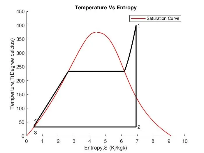
Fig. Graph of Temperature vs Entropy
2) Graph of Enthalpy vs Entropy
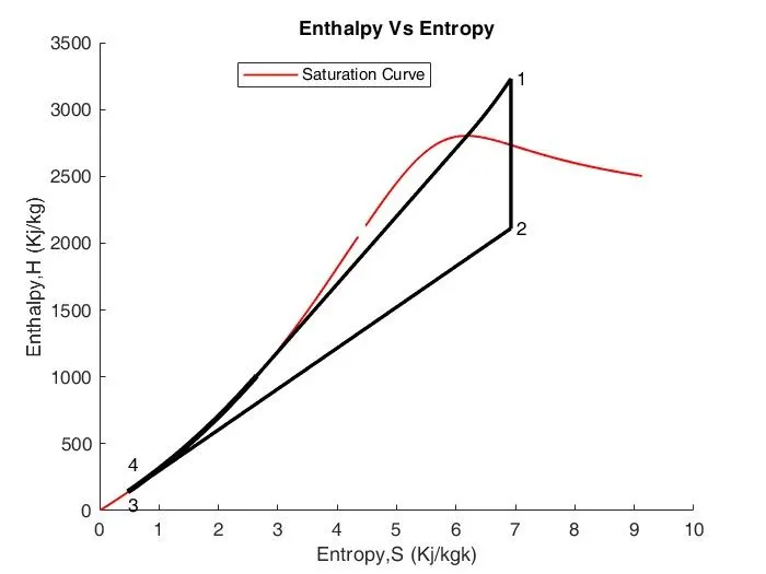
Fig.Graph of Enthalpy vs Entropy
3) Command Window Results
Conclusion:
We are successfully getting the Rankine Cycle Simulation of Steam Turbine , by using Various Input Parameters. Also we are Geting The 'T-S' and ' H-S' Plots.
Refrences:
https://en.wikipedia.org/wiki/Rankine_cycle
en.wikipedia.org/wiki/Steam_turbine
https://www.sciencedirect.com/topics/engineering/steam-turbines