Week 3 - Solving second order ODEs

Aim:

Solving second order differential equation of a simple pendulum and using animation to show damping effect of simple pendulum.

Major Objective:

• To create MatLab function code for solving ordinary differential equation.
• To plot the angular displacement and angular velocity vs time for the problem of simple pendulum.
• To make an animation of stimulation of simple pwndulum.

Theory:

In Mathematics, a differential equation is an equation with one or more derivatives of a function. The derivative of the function is given by dy/dx. In other words, it is defined as the equation that contains derivatives of one or more dependent variables with respect to one or more independent variables.

Second Order Differential Equation:

The order of a differential equation is the highest-order derivative that it involves. Thus, a second order differential equation is one in which there is a second derivative but not a third or higher derivative.

To solve the equation in the MATLAB by using ‘ode45’ the equation needs to be converted from 2^nd order partial differential equation to 1^st order differential equation.

Consider `\theta = \theta1`

Then new equation of motion can be written as:

`(d^2\theta1)/(dt^2)+b/m(d\theta1)/dt+g/Lsin\theta1=0`

Consider,

`(d\theta1)/dt=\theta2`

Therefore, new equation can be written as:

`(d\theta^2)/dt+b/m\theta2+g/Lsin⁡\theta1=0`

Which leads to:

`(d\theta^2)/dt=-b/m\theta2-g/Lsin⁡\theta1`

The resultant first order equation will be:

`\theta′1= \theta2`

`\theta′2=−b/m\theta2−g/Lsin\theta1`

Function Code:

This is the function code used for the main ode code.

function [dtheta_dt] = ode_func(theta,b,m,g,L,t)
    theta1=theta(1); % Assign value theta(1) to thetal
    theta2=theta(2); % Assign value theta(2) to theta2
    dtheta1_dt= theta2;
    %derivation of theta 1 and theata 2 
    dtheta2_dt= (-b/m)*theta2-(g/L)*sin(theta1);
    % creating array of dtheta dt for function which is coloumn matrix 
    [dtheta_dt] = [dtheta1_dt;dtheta2_dt];
end  

Main MATLAB Code:

Here below show the code for the solving, ploting, and making animation.

In this the main code the input values are:

1. L = 1 m
2. m = 1 kg
3. b = 0.05
4. g = 9.81`m/s^2`

close all
clear all
clc
%Input data 
L= 1;                      %meter
m= 1;                      %kg
b=0.05;                    %damping Coefficient 
g=9.81;                    % m/s^2
% Intial condition
theta_0 = [0;4];%1st coloumn represents displacement while 2nd represents velocity
% time span for pendulum
t_span = linspace(0,20,400); %total time taken is 20s where 400 in between values are considered. 
%Solving ade by ode45 
[t,results]= ode45(@(t, theta) ode_func(theta,b,m,g,L,t),t_span,theta_0);
%Plotting for analysing pandulum transient behavior and pendulum animation

figure(1) % Creating figure window for plotting
plot(t,results (:,1)) %Plotting a graph for tise vs results(1) which is displacement 
hold on               %Hold the figure window 1 For furture plotting 
plot(t, results (:,2))%Plotting a graph for time vs results(1,2) which is velocity
xlabel('Time')        %Naned x-axis as Time
ylabel('Angular Displacement/ Angular Velocity') %Named y-axis as Angular Displacement/Angular Velocity
legend('Angular Displacement','AngularVelocity')
grid on 
hold off 

figure(2)
plot(results(:,1), results(:,2))
xlabel ('position')
ylabel ('Angular velocity')
legend('Angular velocity')


theta2 = results(:,1) 
ct=1;
for i =1: length(theta2)
theta3 = theta2(i);
% for fixed bar and movung bar of a pendulum
x0 = 0;
y0 =0;
x1 = 1*sin(theta3);
y1 = -1*cos(theta3);
% giving axis, color for the pendulum bob

figure(3)
plot([-1.1 1.1],[0,0], 'linewidth' ,3)
hold on
plot([x0 x1],[y0 y1], 'k', 'linewidth',3)
hold on
plot(x1,y1,'o', 'markers',20,'markerfacecolor','r')
xlabel('x-axis')
ylabel('y-axis')
hold off
grid on
axis ([-1.5 1.5 -1.5 0.5])
% time frame to get the the video
pause(0.003)
M(ct) = getframe(gcf);
ct = ct+1;
end

% Code for mmovie
movie(M)
videofile = VideoWriter('Simple Pendulum.avi', 'uncompressed AVI')
open(videofile)
writeVideo(videofile,M)
close(videofile)

Code Explaination:

1. Initially the input parameter are been entered in the code.
2. The total time is 0 to 20 seconds for 400 values in them.
3. Then finally solve the ode using the function code, later the final code is solved using the ode45 in built matlab function.
4. Now all the various codes are being created as per the required problem
5. Using "VideoWriter" movie/animation is being stored by MATLAB.

Results:

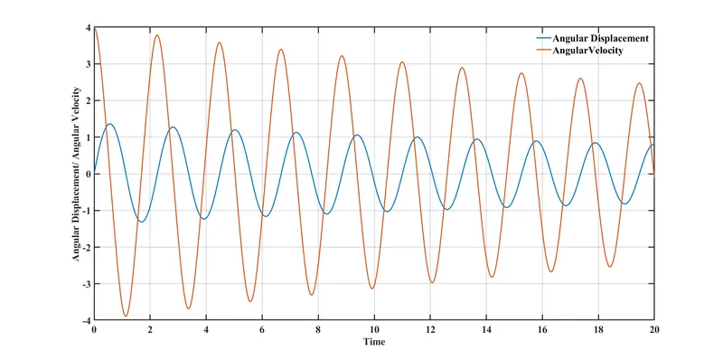
Fig 1.1 Variation of Angular Displacement and Angular Velocity vs Time

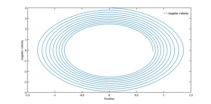
Fig 1.2 Variation of Angular Velocity vs Position

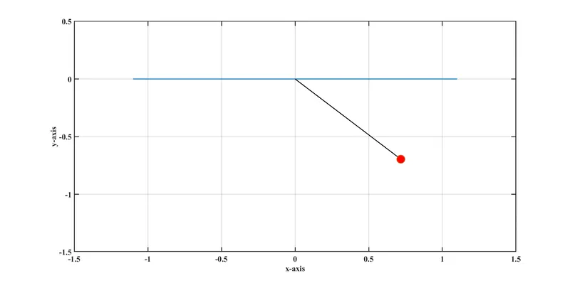
Fig 1.3 Simple Pendulum

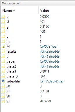
Fig 1.4 Workspace

The fig1.3 show the screenshot of the one frame of the animation. The fig 1.4 shows the different final value of the mathematical calculation performed.

Error:

There was a small error due to change in order for calling function.

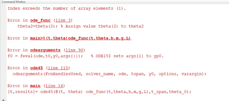
Fig 1.5 Error in command window

Animation for Simple Pendulum:

https://youtu.be/2fseMtWgoME