Project 2 - Rankine cycle Simulator

Aim:

1. To Simulate a Rankine cycle using matlab.
2. Extracting Steam and water properties from Xsteam file.
3. Calculating all the state points of the cycle based on given input data.
4. Plotting the T vs S and H vs S plot.

Theory:

[2]For each process in the vapour power cycle, it is possible to assume a hypothetical or ideal process which represents the basic intended operation and involves no extraneous effects. For the steam boiler, this would be a reversible constant pressure heating process of water to form steam, for the turbine the ideal process would be reversible adiabatic expansion of steam,

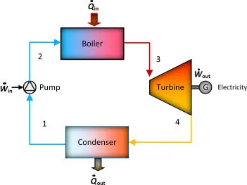
Fig 1.1 Rankine Cycle[1]

for the condenser it would be a reversible constant pressure heat rejection as the steam condenses till it becomes saturated liquid, and for the pump, the ideal process would be the reversible adiabatic compression of this liquid ending at the initial pressure. When all these four processes are ideal the cycle is an ideal cycle, called a Rankine cycle. This is a reversible cycle. Figure 1.1 shows the flow diagram of the Rankine cycle.

Main code for the rankine cycle:

clear all
close all
clc

disp(' RANKINE CYCLE ');                                   
disp('1-2 is Constant pressure heat addition in the boiler');
disp('2-3 is Isentropic Expansion in the Turbine');
disp('3-4 is Constant pressure heat removal in the Condenser');
disp('4-1 is Isentropic compression in the pump');

p1 = 30;
disp('Pressure at turbine inlet, p1(in bar) = 30 bar')
T1 = 400;
disp('Temperature at turbine inlet, T1(in ^\circC) = 400^\circC');
p2 = 0.05;
disp('Pressure at condenser inlet, p2(in bar) = 0.05 bar');

% At State 1
h1 = XSteam('h_pT', p1, T1);        % Extracting Enthalpy at state pt 1
s1 = XSteam('s_pT', p1, T1);        % Similarly

% At State 2
s2 = s1;                            % Isentropic Expansion                
sf2= XSteam('sL_p', p2);            % Saturated Liquid Entropy
sg2 = XSteam('sV_p', p2);           % Saturated Vapour Entropy
x2 = (s2-sf2)/(sg2-sf2);
hf2 = XSteam('hL_p', p2);           
hg2 = XSteam('hV_p', p2);
h2 = hf2 + (x2*(hg2-hf2));

% At State 3
p3 = p2;                            % Constant pressure Heat rejection in Condenser
s3= XSteam('sL_p', p3);
h3 = XSteam('hL_p', p3);

% At State 4
s4 = s3;
p4 = p1;

% Work done by turbine
Wt = h1 - h2;

% Work done to run pump
v3 = XSteam('vL_p', p3);
Wp = v3*(p4 - p3)*100;
h4 = h3 + Wp;

%Net work
Wnet = Wt - Wp;

%Heat into the system
Qin = h1 - h4;

%Heat out of the system
Qout = h2 - h3;

%Thermal efficiency
thermal_eff = (Wnet/Qin)*100;

%Specific Steam Consumption
%SSC = mass flow rate/power
SSC = (3600/Wnet);

% Back Work ratio
BW = (Wp/Wt)


% Calculation of Temperatures at the state points
T3 = XSteam('Tsat_p', p3);
T2 = T3;
Cp4 = XSteam('Cp_ps', p4, s4);
Cv4 = XSteam('Cv_ps', p4, s4);
k = Cp4/Cv4;
T4 = T3/((p3/p4)^((k-1)/k));

%Calculating Temperature, Entropy and Enthalpy at the vapour and liquid line for plotting
T6 = XSteam('Tsat_p', p1);
s5 = XSteam('sL_p', p1);
s6 = XSteam('sV_p', p1);
h5 = XSteam('hL_p', p1);
h6 = XSteam('hV_p', p1);
T5 = T6;


%Plotting the saturation curve
T = linspace(1,375,1000);
for i = 1:length(T)

sf(i) = XSteam('sL_T', T(i));
sg(i) = XSteam('sV_T', T(i));
hf(i) = XSteam('hL_T', T(i));
hg(i) = XSteam('hV_T', T(i));
end

%Plotting T-s diagram
figure(1)
hold on
plot(sf, T, 'r','linewidth',1)
plot(sg, T, 'r','linewidth',1)
plot([s1 s2], [T1 T2], 'b', 'linewidth', 2)
plot([s2 s3], [T2 T3] ,'b', 'linewidth', 2)
plot([s3 s4], [T3 T4], 'b', 'linewidth', 2)
plot([s4 s5], [T4 T5], 'b', 'linewidth', 2)
plot([s5 s6], [T5 T6], 'b', 'linewidth', 2)
sc1 = linspace(s6, s1, 1000);
for l = 1:length(sc1)
 Tc1(l) = XSteam('T_ps', p1, sc1(l));
end
plot(sc1, Tc1, 'b', 'linewidth', 2)
text(s1+0.1, T1, '1')
text(s2+0.1, T2, '2')
text(s3, T3-20, '3')
text(s4, T4+20, '4')
title('Temp vs Entropy plot')
xlabel('Entropy ,S (Kj/kgk')
ylabel('Temperature (^\circC) ')
legend('Saturation curve')


%Plotting h-s diagram
figure(2)
hold on
plot(sf, hf, 'k', 'linewidth', 1)
plot(sg, hg, 'k',  'linewidth', 1)
plot([s1 s2], [h1 h2], 'r', 'linewidth', 2)
plot([s2 s3], [h2 h3], 'r', 'linewidth', 2)
plot([s3 s4], [h3 h4], 'r', 'linewidth', 2)
hc = linspace(h4, h5, 100);
for r = 1:length(hc)
sch(r) = XSteam('s_ph', p1, hc(r));
end
plot(sch,hc, 'r', 'linewidth', 2)
plot([s5 s6], [h5 h6], 'r', 'linewidth', 2)
for m = 1:length(sc1)
hc1(m) = XSteam('h_ps', p1, sc1(m));
end
plot(sc1, hc1, 'r', 'linewidth', 2)
text(s1+0.1, h1, '1')
text(s2+0.1, h2, '2')
text(s3, h3-100, '3')
text(s4, h4 +200, '4')
title('Enthalpy vs Entropy plot')
xlabel('Entropy , S (KJ/kgk) ')
ylabel('Enthalpy , H (KJ/kg)')
legend('Saturation curve','location','northwest')



% Displaying the Results in the Command Window:
disp('Results');
p1 = p1;
T1 = T1;
p2 = p2;
disp('At stage point 1');
n1 = sprintf('P1 is %.3f bar',p1);
disp(n1);
n2 = sprintf('T1 is %.3f C',T1);
disp(n2);
n3 = sprintf('h1 is %.3f kJ/kg',h1);
disp(n3);
n4 = sprintf('s1 is %.3f kJ/kgK',s1);
disp(n4);
disp('At stage point 2');
n5 = sprintf('P2 is %.3f bar',p2);
disp(n5);
n6 = sprintf('T2 is %.3f C',T2);
disp(n6);
n7 = sprintf('h2 is %.3f kJ/kg',h2);
disp(n7);
n8 = sprintf('s2 is %.3f kJ/kgK',s2);
disp(n8);
disp('At stage point 3');
n9 = sprintf('P3 is %.3f bar',p3);
disp(n9);
n10 = sprintf('T3 is %.3f C',T3);
disp(n10);
n11 = sprintf('h3 is %.3f kJ/kg',h3);
disp(n11);
n12 = sprintf('s3 is %.3f kJ/kgK',s3);
disp(n12);
disp('At stage point 4');
n13= sprintf('P4 is %.3f bar',p4);
disp(n13);
n14 = sprintf('T4 is %.3f C',T4);
disp(n14);
n15 = sprintf('h4 is %.3f kJ/kg',h4);
disp(n15);
n16 = sprintf('s4 is %.3f kJ/kgK',s4);
disp(n16);
n17 = sprintf('Wt is %.3f kJ/kg',Wt);
disp(n17);
n18 = sprintf('Wp is %.3f kJ/kg',Wp);
disp(n18);
n19 = sprintf('Wnet is %.3f kJ/kg',Wnet);
disp(n19);
n20 = sprintf('Thermal_efficiency is %.2f Percent',thermal_eff);
disp(n20);
n21 = sprintf('SSC is %.2f kg/kWh',SSC);
disp(n21);
n22 = sprintf('Back work ratio is %.3f ',BW);
disp(n22);

Code Explaination:

1. Initially the code for rankine cycle start with inputing of the given data to it.
2. Extraction of multiple thermodynamic properties are been extracted of water and steam from the steam table given in Xsteam file.
3. Using the mathematical calculation the net work output and back work ratio is been calculated.
4. Futher the plot T-s and H-s diagram for the given plots are been made.
5. In the end shows the display of all the calculated parameter.

Results:

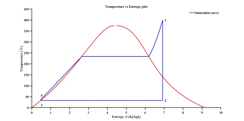
Fig 1.2 Temperature vs Entropy (T-s) diagram

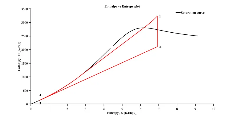
Fig 1.3 Enthalpy vs Entropy (H-s) diagram

Fig 1.2 show the variation of Temperature and Entrpy of the rankine cycle. Where the temperature pt 1 value is 400 `\circ`C, pt 2 value 32.875 `\circ`C, pt 3 value is 32.875 `\circ`C, and the pt 4 value is 36.935 `\circ`C. Where as the fig 1.3 shows the variation of Enthalpy to Entropy leading the various value of Enthalpy at pt 1, pt 2, pt 3, and pt 4 are 3231.571 kJ/kg, 2110.708 kJ/kg, 137.765 kJ/kg, and 140.776 kJ/kg respectively.

Command Window:

Below show the result from the command window:

RANKINE CYCLE
1-2 is Constant pressure heat addition in the boiler
2-3 is Isentropic Expansion in the Turbine
3-4 is Constant pressure heat removal in the Condenser
4-1 is Isentropic compression in the pump
Pressure at turbine inlet, p1(in bar) = 30 bar
Temperature at turbine inlet, T1(in ^\circC) = 400^\circC
Pressure at condenser inlet, p2(in bar) = 0.05 bar

BW =

0.0027

Results
At stage point 1
P1 is 30.000 bar
T1 is 400.000 C
h1 is 3231.571 kJ/kg
s1 is 6.923 kJ/kgK
At stage point 2
P2 is 0.050 bar
T2 is 32.875 C
h2 is 2110.708 kJ/kg
s2 is 6.923 kJ/kgK
At stage point 3
P3 is 0.050 bar
T3 is 32.875 C
h3 is 137.765 kJ/kg
s3 is 0.476 kJ/kgK
At stage point 4
P4 is 30.000 bar
T4 is 36.935 C
h4 is 140.776 kJ/kg
s4 is 0.476 kJ/kgK
Wt is 1120.863 kJ/kg
Wp is 3.011 kJ/kg
Wnet is 1117.852 kJ/kg
Thermal_efficiency is 36.17 Percent
SSC is 3.22 kg/kWh
Back work ratio is 0.003

Workspace:

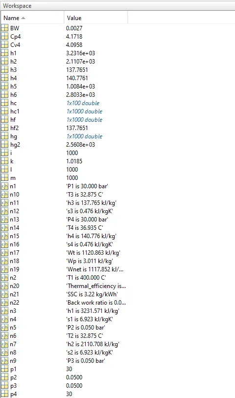
Fig 1.4 Workspace part 1

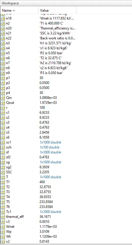
Fig 1.5 Workspace part 2

Fig 1.4 and fig 1.5 show the workspace value that are been obtained.

Refrence:

1. ars.els-cdn.com/content/image/3-s2.0-B9780128099438000029-f02-19-9780128099438.jpg
2. Engineering Thermodynamic : P.K Nag
3. Internal Combustion Engine : V. Ganesan