Aim :
To write a program to simulate the transient behaviour of a simple pendulum and to create an animation file.
Objective :
1.To simulate the motion between 0-20 sec,for angular displacement=0,angular velocity=3 rad/sec at t=0.
2.To solve second order ODE of a simple pendulum with damping using MATLAB ode45 function.
3.To create an animation of pendulum motion using MATLAB.
Equations :
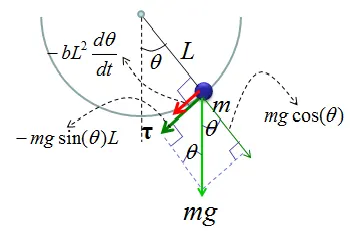
`(d^2(theta))/dt^2+b/m(d(theta))/(dt)+g/lsintheta=0`
Here
`theta`=Angle of pendulum in rad
l=length of pendulum in m
m= mass of pendulum in kg
b=damping coefficient in Ns/m
g= acceleration due to gravity in m/s^2
`(d(theta))/dt=``omega`
`(d^2(theta))/dt^2=alpha`=Angular acceleration in rad/sec^2
Reducing the equation for solving :
`theta=theta_1`
`theta_2=(d(theta_1))/dt=(d(theta))/dt`
Hence
`(d(theta_1))/dt=theta_2`
`(d(theta_2))/dt=-b/mtheta_2-g/lsintheta_1`
MATLAB Program
MATLAB function for ODE45 equation :
%theta=Angle of pendulum in rad
%l=length of pendulum in m
%m= mass of pendulum in kg
%b=damping coefficient in Ns/m
%g= acceleration due to gravity in m/s^2
function [dtheta_dt]=ode_func(t,theta,b,g,l,m)
theta1=theta(1);
theta2=theta(2);
dtheta1_dt=theta2;
dtheta2_dt=-(b/m)*theta2-(g/l)*sin(theta1);
dtheta_dt=[dtheta1_dt;dtheta2_dt];
end
Solving second order ODE of the simple pendulum using MATLAB program :
%solving second order ODE simulation of transient behaviour of a pendulum
clear all
close all
clc
%Inputs
b=0.05; %damping coefficientin Ns/m
g=9.81; %acceleration due to gravity in m/s^2
l=1; %length of pendulum in m
m=1; %mass of pendulum in kg
%Initial condition
theta_0=[0;5];
%time points
t_span=linspace(0,10,500);
%solve ODE
[t,results]=ode45(@(t,theta) ode_func(t,theta,b,g,l,m),t_span,theta_0);
%plotting
xlabel('time t in sec')
ylabel('Angular Displacement')
title('Simple Pendulum with Damping')
figure(1)
hold on
plot(t,results(:,1))
plot(t,results(:,2))
hold off
%to animate the pendulum
t_span=results(:,1);
ct=1;
for i=1:length(t_span)
t_span1=results(i,1);
x0=0;
y0=0;
x1=l*sind(t_span1);
y1=-l*cosd(t_span1);
figure(2);
plot([x0,x1],[y0,y1],'color','b','linewidth',3);
hold on
plot([0.2 -0.2],[0 0],'color','k','LineWidth',4);
plot(x1,y1,'marker','o','color','g','markersize',30,'markerfacecolor','g');
axis([-1 1 -1.5 0.1]);
hold off
M(ct)=getframe(gcf);
ct=ct+1;
end
movie(M)
videofile=VideoWriter('Pendulum.avi','Uncompressed AVI');
open(videofile);
writeVideo(videofile,M);
close(videofile);
Results :
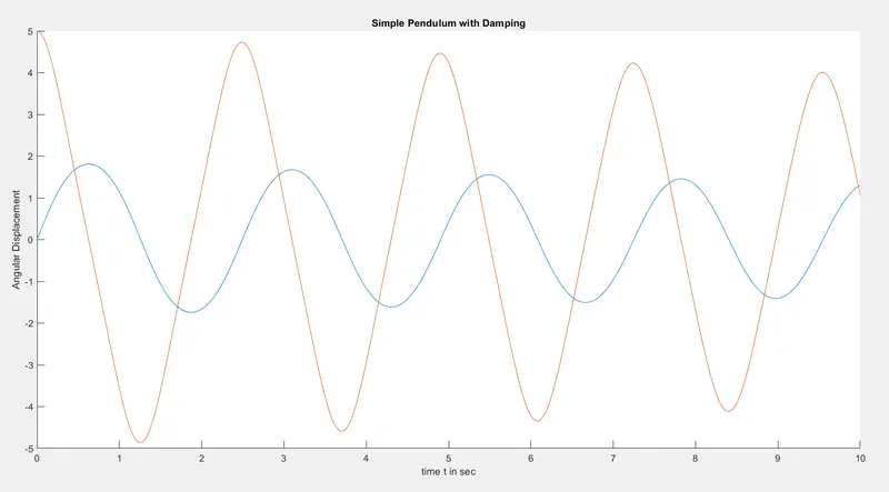
It is evident how the displacement and angular velocity of the bob is affected due to the damper, which is an external force that acts on the system. The higher the damping coefficient, the quicker the motion of the oscillator comes to rest, however due to the low damping coefficient, the motion of the bob will continue much beyond 20 seconds, as is observable from the figure above.
The Animation can be viewed by clicking this link :