Air Standard Cycle

Aim :

To create a PV diagram and the thermal efficiency of the engine using MATLAB.

Objective :

1.To create a PV diagram plots

2.To calculate the thermal efficiency of the engine.

Theory :

The Otto Cycle is named after Nikolaus Otto (1832–1891, German) who is credited as the first creator of a petroleum fuel based internal combustion engine operating under a four stroke cycle.It is one of the most common thermodynamic cycles found in automobile engines and describes the functioning of a typical spark ignition piston engine.

P-V diagram:

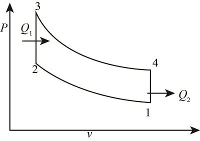
Description of the processes is given as follows:

Process 1-2:

-Isentropic compression of the working fluid occurs as the piston moves from bottom dead center (BDC) to top dead center (TDC).

Process 2-3:

-Here, with the SI, a rapid burning occurs inside the piston; therefore, the heat addition (Q1) takes place at the constant volume(v2=v3).

Process 3-4:

-In this process, the working fluid expands isentropically and produces the useful work for the cycle.

Process 4-1:

-Heat removal at constant volume (v4=v1). In practical applications, the heat (Q2) is removed by expelling the exhaust gas to the atmosphere.

Thermal efficiency :

The efficiency of a heat engine measured by the ratio of the work done by it to the heat supplied to it.

`eta=1-(t_4-t_1)/(t_3-t_2)`

Mathematical equation:

The volume of engine with respect to the rotation :

`v/v_c=1/2(cr−1)[R+1−cosθ−(R^2−sin^2θ)^(1/2)]`

Here,

`v_c=v_(swept)/(cr-1`=clearance volume

`v_swept=(pi/4).(boRe)^2.(stroke)`

compression ratio = cr = 12

`R=L/a`

L=length of connecting rod=con_rod=0.15

a=crank radius=`(stroke)/2`

`theta=`angle of rotation

bore=radius of bore=0.1

stroke=radius of stroke=0.1

Inputs :

`gamma=1.4`

p1=pressure at state1=101325

t1=temperature at state1=500K

t3=temperature at state3=2300K

v1=volume at state1=`v_(swept)+v_c`

v2=volume at state2=`v_c`

p2=`p1.cr^gamma`=pressure at state2

t2=`(p2.v2.t1)/(p1.v1)`p2.v2.t1p1.v1">=temperature at state2

v3=v2

p3=`(p2.t3)/(t2)`p2.t3t2">=pressure at state3

v4=v1

p4=pressure at state4=`p3.((v3)/(v4))^gamma`

t4=temperature at state4

Efficiency of Otto Cycle:

`eta=1-(t4-t1)/(t3-t2)`

MATLAB Program :

ENGINE KINEMATICS MATLAB FUNCTION :

%program to simulate otto cycle volume trace

function[volume_trace]=engine_kinematics(bore,stroke,con_rod,cr,start_crank,end_crank)

a=stroke/2;

R=con_rod/a;

%calculating swept volume and clearance volume

v_swept=(pi/4)*bore^2*stroke;

v_clearance=v_swept/(cr-1);

theta=linspace(start_crank,end_crank,100);

term1=0.5*(cr-1);

term2=R+1-cosd(theta);

term3=(R^2-sind(theta).^2).^0.5;

volume_trace=(1+term1*(term2-term3)).*v_clearance;

SIMULATE THE MATLAB PROGRAM OF OTTO CYCLE :

%program to simulate the otto cycle

clear all

close all

clc

%inputs

gamma=1.4;

t3=2300;

%state variables at state point1

p1=101325;

t1=500;

%engine geometric parameters

bore=0.1;

stroke=0.1;

con_rod=0.15;

cr=12;

%calculating the swept volume and clearance volume

v_swept=(pi/4)*bore^2*stroke;

v_clearance=v_swept/(cr-1);

v1=v_swept+v_clearance;

v2=v_clearance;

%state variables at state point2

%p2v2^gamma=p1v1^gamma | p2=p1(v1/v2)^gamma=p1*cr^gamma

p2=p1*cr^gamma;

%p1v1/t1=p2v2/t2 | t2=p2v2*t1/(p1*v1)

t2=p2*v2*t1/(p1*v1);

constant_c1=p1*v1^gamma;

v_comp=engine_kinematics(bore,stroke,con_rod,cr,180,0);

p_comp=constant_c1/(v_comp.^gamma);

%state variables at state point3

v3=v2;

%p3v3/t3=p2v2/t2 | p3=p2*t3/t2

p3=p2*t3/t2;

%state variables at state point4

v4=v1;

%p3v3^gamma=p4v4^gamma | p4=p3(v3/v4)^gamma

p4=p3(v3/v4)^gamma;

%p3v3/t3=p4v4/t4 | t4=p4*v4*t3/(p3*v3)

t4=p4*v4*t3/(p3*v3);

constant_c2=p3*v3^gamma;

v_exp=engine_kinematics(bore,stroke,con_rod,cr,0,180);

p_exp=constant_c2/(v_exp.^gamma);

etaOtto=1-((t4-t1)/(t3-t2));

%plotting

figure(1)

hold on

plot(v_comp,p_comp,'color','m','linewidth',1);

plot([v2 v3],[p2 p3],'color','c','linewidth',1);

plot(v_exp,p_exp,'color','g','linewidth',1);

plot([v4 v1],[p4 p1],'color','r','linewidth',1);

plot(v1,p1,'.','color','b');

plot(v2,p2,'.','color','b');

plot(v3,p3,'.','color','b');

plot(v4,p4,'.','color','b');

annotationStr=strcat('otto cycle efficiency=',sprintf('%0.4f',etaOtto));

annotation('textbox','string',annotationStr);

legend('Isentropic Compression','Constant Volume Heat Addition','Isentropic Expansion','Constant Volume Heat Rejection');

title('OTTO CYCLE')

xlabel('PRESSURE')

ylabel('VOLUME')

hold off

Explanation :

step 1 : Trace the volume of the engine using ENGINE KINEMATICS MATLAB FUNCTION.

step 2 : Calculate the state points using mathematical formulas.

step 3 : Calculate the path values of isentropic compression and expansion.

step 4 : Calculate the efficiency of the otto cycle.

step 5 : plot state points and path lines.

Results :

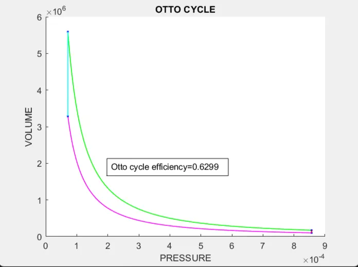
Conclusion :

Hence, P-V diagram plot was created and thermal efficiency of otto cycle was calculated.