Week 3 - Solving second order ODEs

Aim: To Solve the 2nd order ODE System and to simulate the motion of Simple Pendulum using Matlab.

Theory:

Generally Ordinary Differential Equations (ODE) evaluated for the system gives transient behavoiur of that sytem. One such example is Simple pendulum with damping.

Simple Pendulum with damping:

A simple pendulum is explained as a point mass (bob) attached to the one end of the non-stretchable and massless string while other end is fixed to some point, about which it is allowed to swing back and forth about its equillibrium position. Whenever the viscous dragforce (damping force) of the medium (here air) is considered for evaluation of motion parameters the then it is simple pendulum with damping.

The ODE for simple pendulum with damping is stated as follows:

`ddot\theta+(b/m) dot\theta+ (g/L) sin(\theta)=0`

where

`\theta -"Angular displacement of Mass from Equilibrium position "`;

`dot\theta -"Angular velocity "`;

`ddot\theta -"Angular acceleration "`;

`b -"Coefficient of Damping "`;

`m -"Mass of the bob "`;

`g -"Acceleration due to gravity "`;

`L -"Length of the string of the pendulum "`

Assumptions:

1. String is non-stretchable and massless.
2. Bob has point mass.
3. Angular Displacement (`\theta`) is small such that `sin\theta rarr \theta` (in radians).

Figure:

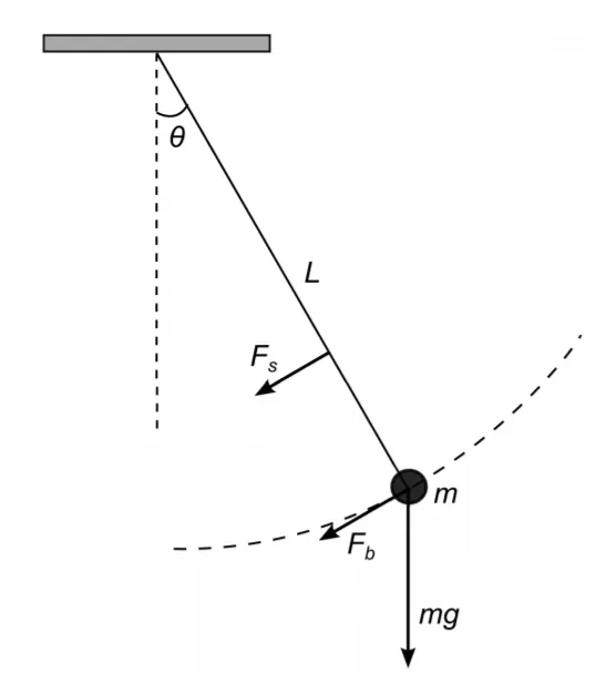
Figure shows simple pendulum with damping (`F_s` & `F_b` are drag forces on string and bob repectively).

Objectives:

1. To Write the MATLAB code to solve the ODE for Simple pendulum with damping using given initial conditions.
2. To write a code to make the animation of Pendulum motion. To save and to share the Youtube link of the animation.
3. To plot the graph of angular displacement and angular velocity with the time.

Process:

1. Defined timpespan using linspace function for 20 seconds. Stated intial conditions in `"theta_0" variable as initial angular displacement is 0 radians and initial angular velocity as 3 radians per second.
2. Stated given parameters with their values.
3. Solved ODE using inbuilt solver ode45 and fuction to solve ODE.
4. Linetracing and animation frames for Pendulum saved. Animation Video uploaded on You tube.
5. Graph ploted for Angular displacement ,angular velocity and angular accelration with respect to time.

Main Code:

clear all
close all
clc

% Solving ODEs of second order for pendulum with damping
t=linspace(0,20,1000);    %Simulation Timespan
theta_0=[0,3];            % Initial conditions angular disp=0 & angular vel=3rad/sec at t=0.

%Parameters
L=1;          % Length in meters
g=9.81;       % Gravitional acceleration in m/s^2
b=0.05;       % Damping Coeff
m=1;          % mass in kg
ct=1;         %counter for aniation frames 

%Solving ode by using ode45
[t,y]=ode45(@(t,theta)ode_pendulum_damping(t,theta,L,g,b,m),t,theta_0);
%calculate acceleration
y(:,3)= (-(b/m).*y(:,2))-((g/L).*y(:,1));

%plotting
subplot(3,1,1) 
plot(t,y(:,1),'color','r','linewidth',1)%Plot of Angular displacement vs time
hold on
plot(t,y(:,2),'color','b','linewidth',1)%Plot of Angular velocity vs time
hold on
plot(t,y(:,3),'color','g','linewidth',1)%Plot of Angular acc vs time
hold on
p1=plot(t,y(:,1),'o','MarkerFaceColor','r');%tracing point for Angular Displacement
p2=plot(t,y(:,2),'o','MarkerFaceColor','b');%tracing point for Angular Vel
p3=plot(t,y(:,3),'o','MarkerFaceColor','g');%tracing point for Angular Acc
hold off
xlabel('time-(sec)')
ylabel('(\theta) & (\omega) &(\alpha)') 
legend('(\theta)-(rad)','(\omega)-(rad/s)','(\alpha)-(rad/s^2)')
grid on 
grid minor

theta2=y(:,1);
for i=1:length(theta2)  
    p1.XData=t(i);p1.YData=y(i,1); %tracer coordinates for Angular Displacement
    p2.XData=t(i);p2.YData=y(i,2); %tracer coordinates for Angular Vel
    p3.XData=t(i);p3.YData=y(i,3); %tracer coordinates for Angular Acc
    drawnow                        % As length of theta2 & t is same hence tracing synchronised   
   
    theta_x=theta2(i);
    X0=0;                  %Linkage Fixed point x coordinate
    Y0=0;                  %Linkage Fixed point y coordinate
    X1=L.*sin(theta_x);    %Pendulum bob center point x coordinate
    Y1=-L.*cos(theta_x);   %Pendulum bob center point y coordinate
    
    %Plotting the pendulum frame
    subplot(3,1,(2:3))
    plot([-0.5,0.5],[0,0],'color','k','linewidth',5); % Support surface
    hold on
    plot([X0,X1],[Y0,Y1],'color','b','linewidth',2);  % Link of pendulum 
    hold on
    plot(X1,Y1,'o','markers',15,'markerfacecolor','r'); % Bob of pendulum
    t_string=num2str(t(i));              % Time as number converted to string to display
    text(X1,(Y1-0.2),t_string,'color','k','FontSize',15) % To Display Time of simulation 
    hold off
    grid on
    grid minor
    axis([-1.5,1.5,-1.5,0.5]); %frame boundaries
    M(ct)=getframe(gcf); %Capturing Current frame with getframe command
    ct=ct+1;             % Loop counter increament
end

movie(M); % Stiching all the frames to array M to creat an animation
%Cteating uncompressed file called Forward_kinematics_2.avi and assigning it to the
%variable named videofile 
videofile=VideoWriter('Simple_Pendulum.avi','Uncompressed AVI');
open(videofile)
writeVideo(videofile,M)
close(videofile)

figure(2) 
plot(t,y(:,1),'r',t,y(:,2),'b',t,y(:,3),'g') % Seperate Plot of Angular displacement,vel& acc vs time
xlabel('time-(sec)')
ylabel('Angular Disp(\theta)& Angular Vel(\omega)& Angular Acc(\alpha)')%('(\theta)-(rad)&(\omega)-(rad/s)&(\alpha)-(rad/s^2)')
legend('(\theta)-(rad)','(\omega)-(rad/s)','(\alpha)-(rad/s^2)')
grid on 
grid minor
saveas(gcf,'Angular displacement,velocity & acceleration vs time','jpg') % saving figure (2)

Function Code: (ode_pendulum_damping.m)

function [theta_dot]=ode_pendulum_damping(t,theta,L,g,b,m)

theta_dot(1)=theta(2);                              % Angular velocity 
theta_dot(2)=(-b/m).*theta(2)-(g/L).*sin(theta(1)); % Angular accelration
theta_dot=[theta_dot(1);theta_dot(2)];              % theta_dot array 

end

Animation You tube link: https://youtu.be/vEXayDehNcE

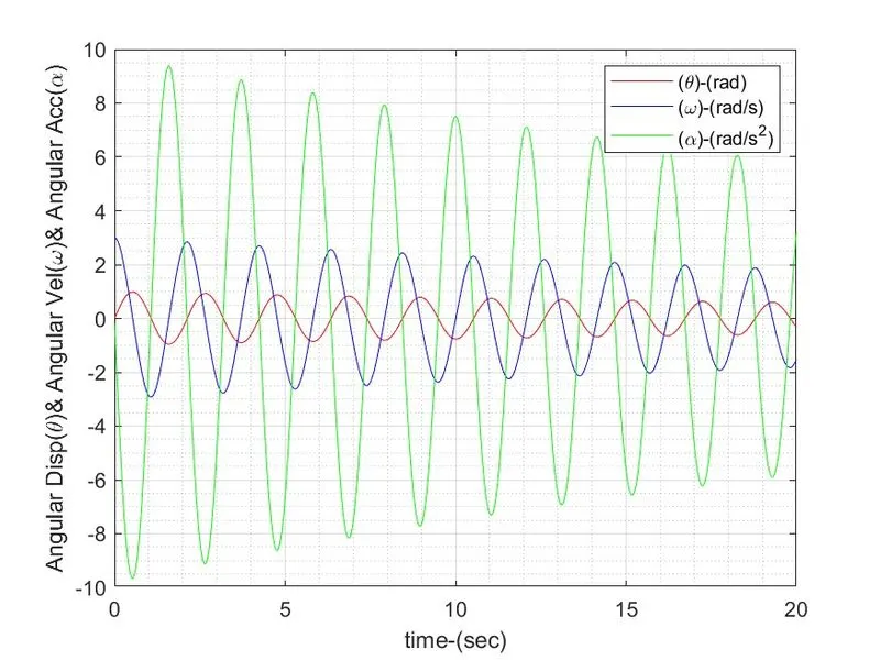
Graph: Angular displacement ,angular velocity & angular acceleration with time.

Conclusions:

1. Due to damping the magnitudes of angular dispalcement, angular velocity and angular accelration are decreasing.
2. Due to low damping coefficient the pendulum does not stop within 20 seconds.