Week 3 - Solving second order ODEs

Aim:

To write a program in Matlab software to simulate the motion of the pendulum and the damping coefficient of displacement and velocity of the pendulum.

Objective:

The objective of the program is to create sine wave of damping coefficient of angular displacement and angular velocity of the pendulum.

Then to create an animation video for the periodic motion of oscillating motion of the pendulum by solving one order ODE.

Diagram:

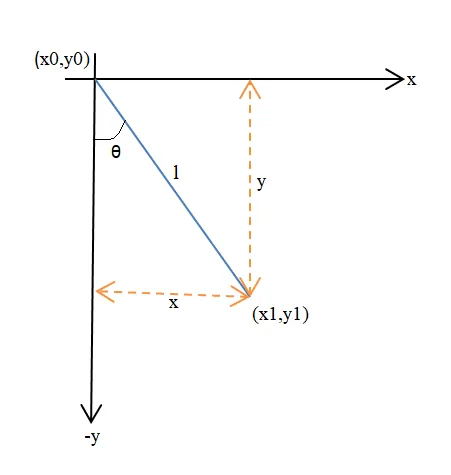
Graphical representation of pendulum are,

Equations:

From the graphical representation the equation of the coordinates are derived. They are,

x0 = 0

y0 = 0

sin`theta`=`frac{x}{l}` => x = l*sin`theta`

cos`theta`= `frac{y}{l}`=> -y = l*cos`theta`

Pendulum differential equation: Daming case

The represented Ordinary Differential Equation for the motion of the simple pendulum with damping

`frac{d^2(theta)}{dt^2}+frac{b}{m}*frac{d(theta)}{dt}+frac{g}{l}*sin(theta)=0`

This equation cannot be solved directly in matlab, so that we have to breakdown the second order ODE into the series of first order ODE,

Displacement `theta = theta1`

Velocity `frac{d^2theta}{dt^2}= theta2`- (1)

`frac{d^2(theta1)}{dt^2}+frac{b}{m}*frac{d(theta1)}{dt}+frac{g}{l}*sin(theta1)=0`

`frac{d}{dt}(frac{d theta1}{dt})+frac{b}{m}*theta2+frac{g}{l}*sin(theta1)=0`

`frac{d}{dt}*(theta2)+frac{b}{m}*theta2+frac{g}{l}*sin(theta1)=0`

`frac{d theta2}{dt}= frac{-b}{m}*theta2-frac{g}{l}sin theta1` - (2)

from that the second order ODE is break down into two first order ODE

Inertia force = m*`frac{d^2t}{dt^2}`

Damping force = b*`frac{d theta}{dt}`

Gravity force =`frac{g}{l}*sin theta1`

where,

g = gravity in m/s2,

l = length of the pendulum in m,

m = mass of the ball in kg,

b=damping coefficient

Explaination:

Simple pendulum:

The simple pendulum consists of a mass of a object hanging at the end of the string having a length and the string is fixed at a point of (x) coordinates. The pendulum is displaced at an initial angle and released, the pendulum will swing front and backward with periodic motion.

ODE45:

The ODE45 is an inbuilt function, where ODE solvers can solve systems of equations or problems that involve a mass matrix.

Procedure:

• By provilding all the inputs for the simple pendulum, create a function for the equation of the ODE.
• Create a time span for the varying position of the oscillating pendulum.
• Then identify the time span in the for loop command .
• Then provide all the coordiates of the derived equations
• After that by using the movie command to create the animation.

Code for simple pendulum:

function [dtheta_dt] = ode_func (t,theta,b,g,l,m) 
theta1 = theta(1);
theta2 = theta(2);
dtheta1_dt = theta2;
dtheta2_dt = (-b/m)*theta2 - (g/l)*sin(theta1);
[dtheta_dt] = [dtheta1_dt; dtheta2_dt];
end

clear all
close all 
clc
%pendulum inputs
b = 0.05;     %b = damping coefficient
g = 9.81;     %g = gravity in m/s^2
l = 1;        %l = length of pendulum in m    
m = 1;        %m = mass of the ball in kg

%initial conditions
%Angular displacement = 0
%Angular velocity = 5
theta_0=[0;5];
t_span = linspace(0,20,200);

[t,results]=ode45(@(t,theta) ode_func(t,theta,b,g,l,m),t_span,theta_0);
%plotting
figure(1)
hold on
plot(t,results(:,2))
plot(t,results(:,1))
xlabel('time')
ylabel('plot')
legend('velocity','displacement')
THETA1=results(:,1);
ct = 1;
for i =1:length(t_span)
    
    %coordinates
    x0 = 0;
    y0 = 0;
    x1 = l*sin(THETA1(i));
    y1 = -l*cos(THETA1(i));
    
    figure(2)
    plot([x0 x1],[y0 y1],'linewidth',3,'color','r')
    hold on
    plot(x1,y1,'Marker','.','Color','y','MarkerSize',70)
    axis([-1.5 1.5 -1.5 1.5])

    M(ct)=getframe(gcf);
    ct = ct+1;
    hold off
end
%movie creation
movie(M);
videofile=VideoWriter('pendulum movie','Uncompressed AVI');
open(videofile)
writeVideo(videofile,M)
close(videofile)

Output:

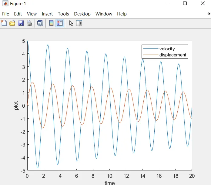
Angular displacement and angular velocity

Result:

The result is obtained for the simulation of motion of the pendulum. Then the animation video is also created for the pendulum motion.

the link is attached below for the animation video of the pendulum motion.

https://youtu.be/SjW9gOYVMug