Week 3 - Solving second order ODEs

OBJECTIVE: To write a program in PYTHON that solves the following ODE. This ODE represents the equation of motion of a simple pendulum with damping

In the above equation,

g = gravity in m/s2,

L = length of the pendulum in m,

m = mass of the ball in kg,

b=damping coefficient.

THEORY:

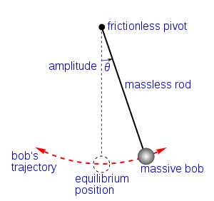
A pendulum is a weight suspended from a pivot so that it can swing freely. When a pendulum is displaced sideways from its resting, equilibrium position, it is subject to a restoring force due to gravity that will accelerate it back toward the equilibrium position. When released, the restoring force acting on the pendulum's mass causes it to oscillate about the equilibrium position, swinging back and forth. The time for one complete cycle, a left swing and a right swing, is called the period. The period depends on the length of the pendulum and also to a slight degree on the amplitude, the width of the pendulum's swing.

From the first scientific investigations of the pendulum around 1602 by Galileo Galilei, the regular motion of pendulums was used for timekeeping and was the world's most accurate timekeeping technology until the 1930s.

INPUTS

L=1 metre,

m=1 kg,

b=0.05.

g=9.81 m/s2.

time = 0-20 sec,

for angular displacement=0,angular velocity=3 rad/sec at time t=0.

Procedure:

• Since the given problem represents a second order differential equation, converting this 2nd order ODE into 1st order ODE by following below steps

theta = theta1

`(d θ) /(d t) = (d θ 1)/( d t)`

`(d θ1^2) /(d t^2) = (d θ 2)/( d t)`

CODE:

import math
import matplotlib.pyplot as plt
import numpy as np 
from scipy.integrate import odeint

#function that return dz/dt
def model(theta,t,b,g,l,m) :

	theta1 = theta[0]
	theta2 = theta[1]
	dtheta1_dt = theta2     #1st ode
	dtheta2_dt = -(b/m)*theta2 - (g/l)*math.sin(theta1)   #2nd ode
	dtheta_dt = [dtheta1_dt,dtheta2_dt]
	return dtheta_dt

b = 0.05
g = 9.81
l = 1
m = 1

#initial condition
theta_0 = [0,3]  #displcement, velocity theta2 = dtheta1/dt

#time points
t = np.linspace(0,20,200)

#solve ode 
theta = odeint(model,theta_0,t,args = (b,g,l,m))


#plot results
plt.plot(t,theta[:,0],'b-',label=r'$\frac{d\theta_1}{dt}=\theta2$')
plt.plot(t,theta[:,1],'r--',label=r'$\frac{d\theta2}{dt}=-\frac{b}{m}\theta_2-\frac{g}{L}sin\theta_1$')
plt.xlabel('time')
plt.ylabel('Plot')
plt.legend(loc='best')
plt.title('2nd order ODE')
plt.savefig('2nd order ode.png')
plt.show()

#animation
ct =1
x0 =0
y0 = 0

for i in theta[:,0]:
	x1 = (math.sin(i))
	y1 = -(math.cos(i))

	filename = 'test%05d.png' %ct
	ct = ct+1

	plt.figure()
	plt.plot([-1,1],[0,0],'b',linewidth =10)
	plt.plot([x0,x1],[y0,y1],'r')
	plt.plot(x1,y1,'o',markersize =20)
	plt.xlim([-1.5,1.5])
	plt.ylim([-1.5,1.0])
	plt.savefig(filename)

Procedure:

• It is always recommended to start the program by using these 4 commands
  import math

import matplotlib.pyplot as plt

import numpy as np

from scipy.integrate import odeint

• Assigning the intial values for theta and line lenghts
• Using ODEINT to solve the ode function for arguments b,g,l,m,theta
• Plotting using plt command
• Assigning xlabel, y label, title for the figure
• Saving the figure wiht filename using SAVEFIG command
• Initiating the animation by starting counter as ct= 1
• Assigning the intial values for the start of pendulum
• The end values of pendulum are calculated using basic math, and - sign is added in the y1 to make sure that pendulum moves in proper direction.
• Assigning values to create the base of pendulum
• Plotting the bob and string of pendulum using plt command.
• Assigning the xlimit and y limit values to makesure the figures are within the same axis.
• Saving all the files with .png format
• creating a animation by using magick command

RESULTS:

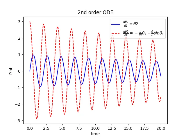
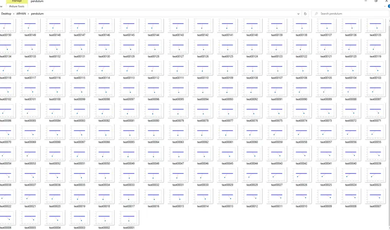
https://drive.google.com/file/d/1aqgCyVJ6DPHBc1yRzgOUHn-CO1O7fUs1/view?usp=sharing

CONCLUSION:

• Python code to solve the ODE is succesfully compiled.
• This ODE represents the equation of motion of a simple pendulum with damping and the animation is succesfully created