Week 3 - Solving second order ODEs

Aim: To solve the following second order ODE(Ordinary Differential Equation) using the MATLAB programming and also simulate a simple pendulum with damping.

`(d^2 θ)/dt=b/m*dθ/dt+g/l sinθ=0`

Governing Equations

`(d^2 θ)/dt=b/m*dθ/dt+g/l sinθ=0`

where,

b = Damping co-efficient of simple pendulum

m = mass of the ball

g = gravitational co-efficient

l = length of the pendulum string

Objective

To develop a program to solve the ODE using the MATLAB programming with the help of the given values and also simulate the simple pendulum with damping

Flow chart

The below flow chart shows the steps following to solve the ODE and simulate the simple pendulum.

Main program:

clear all
close all
clc

% Inputs
m = 1;
l = 1;
g = 9.81;
b = 0.3;

% initial values of displacement and velocity
thetha_0 = [0,3];

%time point
t_span = linspace(0,20,500);

% solve ODE
[t, results] = ode45(@(t,thetha) ode_fun(t,thetha,m,l,g,b),t_span,thetha_0);

% plotting
plot(t,results(:,1))

hold on
grid on

plot(t,results(:,2))
axis([0 22 -4 4])

xlabel('time')
ylabel('amplitude')

% simulation for simple pandulum with damping
ct = 1
for i = 1:length(t)
    result1 = results(i,1);

    x0 = 0;
    y0 = 0;

    x1 = -l*sin(result1);
    y1 = -l*cos(result1);

% plotting for simple pandulum
    figure (2)
    
    plot([-3 3],[0 0],'linewidth',4,'color','b');
    axis([-3.5 3.5 -1.5 0.5])
    
    hold on
    
    plot([x0 x1],[y0 y1],'linewidth',5);

    % for the spherical ball of pandulum
    
   plot(x1,y1,'Marker','o','linewidth',20,'color','r');
   
   hold off
   grid on
   pause(0.03)
   M(ct) = getframe(gcf);
   ct = ct+1; 
   
end

%movie making
movie(M)
videofile = VideoWriter('simple_pandulum_with_damping.avi','Uncompressed AVI');
open(videofile)
writeVideo(videofile,M)
close(videofile)

In the above program, the first part is for input values of the like b, g, l and m and after that the initial value of displacement and velocity are given. Next step is used to divide time of 20 second into the 500 equal parts for that the linspace command is used.

After that the ODE is solving using the ode45 command, which have following syntax

[t,results] = Ode45(@(t,c) ode_function(t,y,arguments),time,initials)

The ode45 takes three inputs, first is integrated function second is time span and third one is initials. This is applicable only on the first order ODE so in the integrated function the second order ODE is converted into first order ODE and solved.

After that the plot for time and amplitude is drown using the plot command. After that the simulation part of the program is started in which first the for loop is used to pick the values one by one for plotting the simple pendulum. For plotting simple pendulum, the coordinates are calculated and after that a movie is made using all the frames made by the simulation of the simple pendulum.

Function program:

function [dthetha_dt] = ode_fun(t,thetha,m,l,g,b)
    thetha1 = thetha(1)
    thetha2 = thetha(2)
    dthetha1_dt = thetha2
    dthetha2_dt = -(b/m)*thetha2-(g/l)*sin(thetha1)
    dthetha_dt = [dthetha1_dt;dthetha2_dt]
end

The above function program is defined to solve the ode function having the function name ode_fun. In the function the second order differential equation is converted to first order differential equation and solved and the result is pass on to the main program.

Result

With the help of the above MATLAB program the below two results are given in which the first plot is about the damping of the SIMPLE PENDULUM showing the graph between the time and the amplitude of the pendulum.

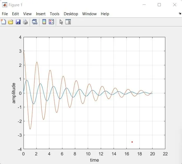
The above graph is showing the movement of the simple pendulum whose amplitude is continuously decreasing with respect to the time.

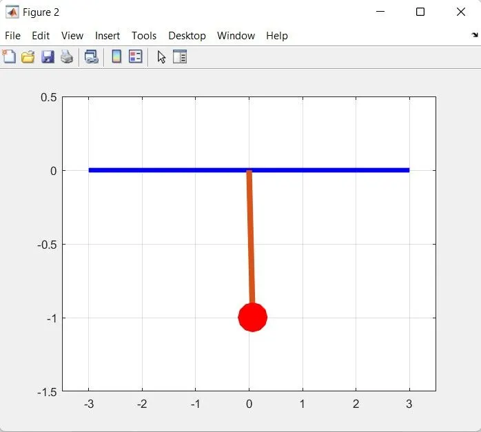
The above image showing the simple pendulum which is simulated using the MATLAB programming and showing the simple pendulum with the damping. The below link is showing the simulation of the Simple pendulum: https://youtu.be/-X1vIwaat_A

Errors in program:

Error1

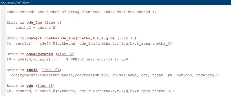
The above error is came due to missing the order of the function values of the ode_fun, So I fix the error by picking the correct order of the values.

Error2

I used the space instead of semi colon so the error is thrown and the error is resolved by replacing the space with the semi colon.

Error3

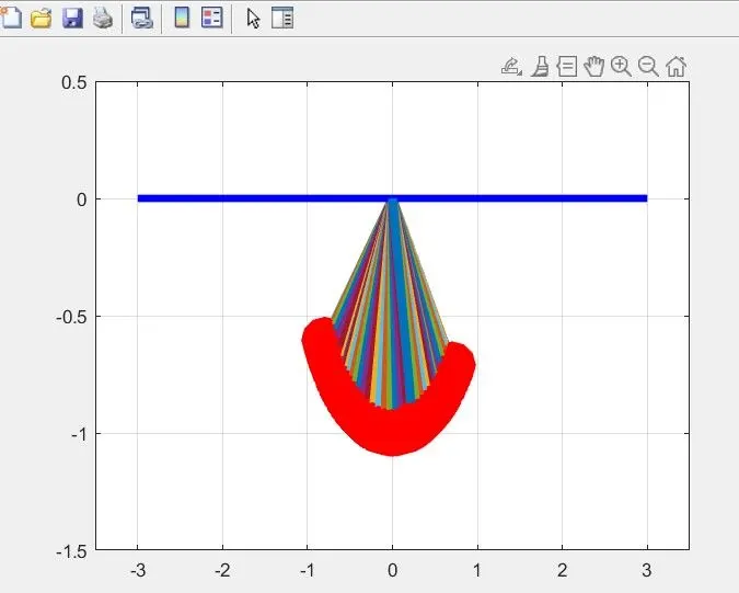
The above plot is shown due to the misplace or removal of the hold off command So to resolve the error I placed the command on their exact place.

Error4

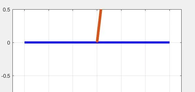
The pendulum is moving upside due to the mistake of taking the coordinate value positive so to resolve this error the coordinate (x1,y1) is taken to be negative.

Conclusion: From the above project, We learn to solve the ODEs (Ordinary Differential Equations) using the MATLAB programming and also learn to simulate the simple pendulum with damping.