Challenge

Project 2 - Rankine cycle Simulator

RRaj Banjara20 Jul 2022

Aim: To create a Rankine cycle simulator using the MATLAB programing and also plot the t-s and h-s diagrams using the data of the Rankine simulator.

Objective:

To display all the stages involved in the Rankine cycle
To calculate all the four stages of the Rankine cycle using the MATLAB and the XSteam file.
To plot the T-s and h-s diagram using MATLAB.

Theory:

The Rankine cycle is an idealized thermodynamic cycle describing the process by which certain heat engine, such as steam turbine or reciprocating steam engines, allow mechanical work to be extracted from a fluid as it moves between a heat source and heat sink.

Heat energy is supplied to the system via a boiler where the working fluid (typically water) is converted into a high-pressure gaseous state (steam) in order to run a turbine. After passing over the turbine the fluid is allowed to condense back into a liquid state by heat rejection before being returned to boiler, completing the cycle. Friction losses throughout the system are often neglected for the purpose of simplifying calculations as such losses are usually much less significant than thermodynamic losses, especially in larger systems.

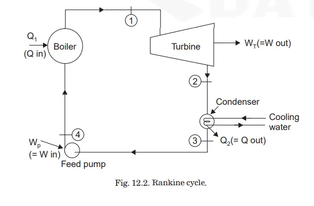
Figure1- Rankine cycle used to run a steam turbine

The Rankine cycle is complete in 4 stages which are shown in the above figure and explain below as following

Stage 1-2: This stage is an isentropic expansion process, in which the vapor generated in the boiler is supplied on the turbine blade and producing power by rotating the turbine blade. In practice, the expansion is limited by the temperature of the cooling medium and by the erosion of the turbine blades by liquid entrainment in the vapor stream as the process moves further.

Stage 2-3: This stage is an Isobaric Heat Rejection. In this stage the vapor-liquid mixture leaving the turbine and enters into the condenser where the vapor-liquid mixture is condensed at low pressure. In a batter quality condenser, the pressure of the vapor is well below the atmospheric pressure and approaching to the saturation pressure of the operating fluid at the cooling temperature.

The amount of heat rejected is calculated by using the following formula:

Where, h2 and h3 are the enthalpies at stage 2 and 3 respectively.

Stage 3-4: This is an isentropic compression process in which the liquid from the condenser is pass to the boiler by the help of the feed pump. The feed pump pumps the liquid to the boiler with negligible thermodynamic changes.

Stage 4-1: This is an isobaric Heat addition process in which Heat is added to the liquid and rise the temperature till the liquid converted into vapor and evaporate.

XSteam Code file:

This file is provided by the skill-Lync to help the candidate to access the steam table data for the Rankine cycle. With the help of the XSteam file we can call the function for finding the values of the stages involved in the Rankine cycle like the enthalpy and entropy of the saturated and superheated vapors.

Main code for Rankine cycle simulator:

clear all
close all
clc

% Showing the rainkine cycle stages
disp('Rankine cycle simulator')
disp('1-2 is the Isentropic Expansion in the Turbine')
disp('2-3 is the constant pressure Heat Rejection in the condenser')
disp('3-4 is the Isentropic Compression in the pump')
disp('4-1 is the constant pressure Heat Addition in the boiler')

% Entering the input pressure and temperature
P1=input('\nvalue Enter the pressure at the Turbine Inlet (in bar):');
T1=input('\nvalue Enter the temperature at the Turbine Inlet (in degree Celsius):');
P2=input('\nvalue Enter the Pressure at the Condenser (in bar):');

disp('RESULTS')


%GETTING Cp and Cv for Xsteam

% For simple problem assume Cp and Cv not affected with temperature

%for vapour
High_CpV = XSteam('CpV_p',P1);
low_CpV = XSteam('CpV_p',P2);
high_CvV=XSteam('CvV_p', P1);
low_CvV=XSteam('CvV_p', P2);


% for liquid
high_CpL= XSteam('CpL_p', P1);
low_CpL=XSteam('CpL_p', P2);
high_CvL=XSteam('CvL_p', P1);
low_CvL=XSteam('CvL_p', P2);

%Getting important parameters from Xsteam 
%for high pressure
Tsat1 = XSteam('Tsat_p', P1);
sg1 = XSteam('sV_p', P1);
sf1 = XSteam('SL_p', P1);
sfg1 = sg1 - sf1;
hf1 = XSteam('hL_p', P1);
hg1 = XSteam('hV_p', P1);
hfg1 = hg1 - hf1;


%Stage 1

disp('At state point 1')

fprintf('P1 is : %f Bar\n', P1)
fprintf('T1 is : %f Deg celsius\n', T1)

%specific enthalpy at stage 1
h1 = XSteam('h_pT',P1,T1);
fprintf('h1 is : %f kJ/kg\n', h1)

%specific entropy at stage 1
s1 = XSteam('s_pT',P1,T1);
fprintf('s1 is : %f kJ/kgK\n\n', s1)

%Stage 2


disp('At state point 2:')
fprintf('P2 is : %f Bar\n', P2)

%specific entropy at stage 2
s2 = s1;
fprintf('s2 is : %f kJ/kgK\n', s2)

%s entropy of liquid and gas from steam table at stage 2
sf2 = XSteam('sL_p',P2);
sg2 = XSteam('sV_p',P2);

%pridecting the value of the dryness factor
if s2<=sg2

    x2 = (s2-sf2)/(sg2-sf2);
else
    x2=1
end

fprintf('x2 is :%f \n', x2)


% if T2 lies in any of the region (superheat,wet or dry )
if(x2<1)
    %dsaturated temperature at satge 2
    Tsat2 = XSteam('Tsat_p',P2)
    T2=Tsat2;  
else 
    %calculation of T2 in superheated region
    %t2 cal by s2=sg2+low_CpV*(log(T2/Tsat2))
    T2=(Tsat2 + 273.15)*exp((s2-sg2)/low_CpV); 
    T2 = T2-273.15;
end    
fprintf('T2 is : %f Deg celsius \n', T2)

% calculation of the enthalpy
if(x2<1)
    %enthalpy at liquid and gas from steam table
    hf2 = XSteam('hL_p',P2);
    hg2 = XSteam('hV_p',P2);

    %calculating enthalpy at stage 2
    h2 = hf2 + (x2*(hg2-hf2));

else
   % calculating enthalpy for superheated steam at stage 2 
    h2 = hg2 + low_CpV*(T2-Tsat2); 
end   
fprintf('h2 is : %f kJ/kg\n', h2)

%stage 3
disp('At state point 3')

P3 = P2;
fprintf('P3 is : %f Bar\n', P3)

%no subcooling assumed
T3 = Tsat2;    
fprintf('T3 is : %f Deg celsius\n', T3)

% specific entropy at stage 3
s3 = XSteam('sL_p',P3);
fprintf('s3 is : %f kJ/kgK\n\n', s3)

%specific enthalpy at stage 3
h3 = XSteam('hL_p',P3);
fprintf('h3 is : %f kJ/kg\n', h3)

%stage 4
disp('At state point 4')

%pressure at stage point 4
P4 = P1;
fprintf('P4 is : %f Bar\n', P4)

%specific entropy at stage 4
s4 = s3;
fprintf('s4 is : %f kJ/kgK\n\n', s4)

% to calculate T4, s4=s3=sf1-high_CpL*ln(Tsat/T4)
 %Use exp instead of Exp to take input as double

 term=exp((sf1-s4)/high_CpL); 
 T4= Tsat1/term;
fprintf('T4 is : %f Deg celsius \n\n', T4)


% volume of the liquid entering in the pump
V3 = XSteam('vL_p',P3);

% work done to run the pump
Wp = V3*(P4-P3)*100;
fprintf('Work by compressor is : %f kJ/kg\n', Wp)

%specific enthalpy at stage 4
h4 = h3 + Wp;
fprintf('h4 is : %f kJ/kg\n', h4)

% work done by turbine
Wt = h1-h2;
fprintf('Work by turbine is : %f kJ/kg\n', Wt)


% net work done
Wnet = Wt - Wp;
fprintf('Net work done is : %f kJ/kg\n', Wnet)

% Heat added to system
Qin = h1-h4;
fprintf('Heat added to the system at boiler is : %f kJ\n',Qin)

% Heat rejected through system
Qout = h2-h3;
fprintf('Heat rejected from the system at condenser is : %f kJ\n',Qout)

% Thermal efficiency

Thermal_efficency = Wnet / Qin ;
fprintf('Thermal efficiency is : %f', Thermal_efficency);
disp('%')

%Specific steam consumption
% SSC = mass flow rate/power
SSC = (3600/Wnet);
fprintf('Specific heat consumption is : %f kg/kWh ', SSC)

%Plotting the saturation  curve

T = linspace(0,375,1000);

for i = 1:length(T)
    H_L(i) = XSteam('hL_T', T(i));
    H_V(i) = XSteam('hV_T', T(i));
    S_L(i) = XSteam('sL_T', T(i));
    S_V(i) = XSteam('sV_T', T(i));
end


% Ploting T - S diagram  
figure(1) 

hold on

plot([s1 s2], [T1 T2], 'r', 'linewidth', 3)
text(s1,T1,' 1')
text(s2,T2,' 2')

plot([s2 sg2], [T2 Tsat2], 'r', 'linewidth', 3)
text(sg2,Tsat2,' 2s')

plot([sg2 s3], [Tsat2 T3], 'r', 'linewidth', 3)
text(s3,T3,' 3')

plot([s3 s4], [T3 T4], 'r', 'linewidth', 3)
text(s4,T4,' 4')

plot([s4 sf1], [T4 Tsat1], 'r', 'linewidth', 3)
text(sf1,Tsat1,' 4s')

plot([sf1 sg1], [Tsat1 Tsat1], 'r', 'linewidth', 3)
text(sg1,Tsat1,' 1s')

plot([sg1 s1], [Tsat1 T1], 'r', 'linewidth', 3)
plot(S_L, T, 'b', 'linestyle','--','linewidth', 3)
plot(S_V, T, 'b', 'linestyle','--','linewidth', 3)

%marking direction
text(s1,(T1+T2)/2,'\vee','HorizontalAlignment','center','color','r')
text((sg2+sf2)/2,T3,'\langle','color','r')
text(s3,(T3+T4)/2,'\wedge','HorizontalAlignment','center','color','r')
text((sf1+sg1)/2,Tsat1,'\rangle','color','r')

title('T-S Diagram of Ideal Rankine Cylce')
ylabel('Temprature (degC)')
xlabel('Specific Entropy (kJ/kgK)')


%h-s diagram using the above data

figure(2)

hold on

plot([s1 s2], [h1 h2], 'r', 'linewidth', 3);
text(s1,h1,' 1')

plot([s2 s3], [h2 h3], 'r', 'linewidth', 1);
text(s2,h2,' 2')

plot([s3 s4], [h3 h4], 'r', 'linewidth', 1);
text(s3,h3,' 3')

plot([s4 s1], [h4 h1], 'r', 'linewidth', 1);
text(s4,h4,' 4')

plot(S_L, H_L, 'b','linestyle','--', 'linewidth', 1.5)

plot(S_V, H_V, 'b','linestyle','--', 'linewidth', 1.5)      

title('H-S Diagram', 'FontSize', 15)
ylabel('Specific Enthalpy (kJ/kg)')
xlabel('Specific Entropy (kJ/kgK)')

The main program is used to calculate all the stages of the Rankine cycle and the enthalpy, entropy and other thermodynamic parameters needed. After calculating the all four stages the T-s and h-s diagrams are plotted by the help of the data calculated in the all four stages.

The above main program is involved all the below stages

Firstly, we display all the stages involved in the Rankine cycle and also enter the input values for the P1, T1 and P2.
After that, the values of the specific heat for constant pressure (Cp) and specific heat for constant volume (Cv) are taken form the XSteam file using the following code

%for vapour
High_CpV = XSteam('CpV_p',P1);
low_CpV = XSteam('CpV_p',P2);
high_CvV=XSteam('CvV_p', P1);
low_CvV=XSteam('CvV_p', P2);


% for liquid
high_CpL= XSteam('CpL_p', P1);
low_CpL=XSteam('CpL_p', P2);
high_CvL=XSteam('CvL_p', P1);
low_CvL=XSteam('CvL_p', P2);

Now some essential parameters are abstracted from the XSteam file like the saturation temperature, sg, sf, hg, hf etc
After that the stage 1 is defined and the specific entropy and enthalpy are calculated using the thermodynamic relations.
In stage 2, The pressure, temperature, entropy, enthalpy and the dryness fraction at stage 2 are calculated for both the saturated and superheated steams using the thermodynamic relations and the XSteam file.
In stage 3, the entropy, enthalpy is calculated using the thermodynamic relations and the XSteam file and also the pressure and temperature calculated.
At stage 4, the pressure, temperature, entropy and enthalpy are calculated using the thermodynamic relations and XSteam file.
After calculating and displaying all four stage parameters the T-s and h-s diagrams are plotted with the title and axis notations.

Error: The errors are described with the solutions below with the screenshot of the command window showing the errors.

Error01:

This error is coming due to extra bracket used so the error is resolved by removing the extra bracket.

Error02:

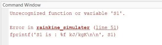
This error is coming because of using ‘S’ instead of ‘s’. so error is resolved by replacing the ‘S’ by ‘s’.

Error03:

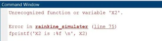
This error is coming because of using ‘X’ instead of ‘x’ so it is resolved by replacing the ‘X’ by ‘x’.

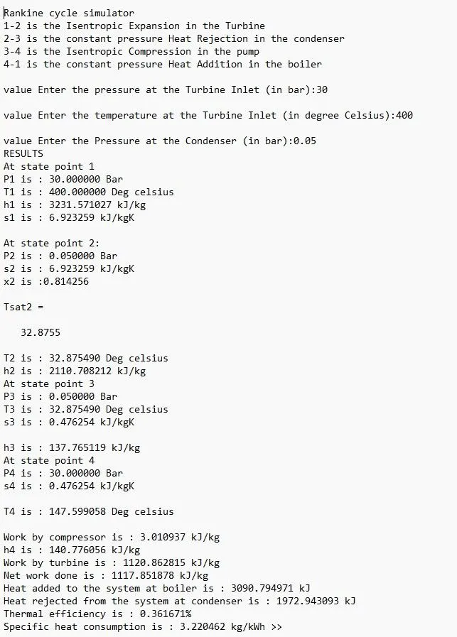
Results:

Plots:

T-s diagram

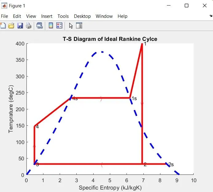
The above diagram is showing the relation between the temperature (T) and the entropy (s) in a Rankine cycle. As shown in the above diagram, there are four stages in the Rankine cycle.

Isentropic expansion
Heat rejection
Isentropic compression
Heat addition

The all 4 stages are shown in the diagram in the red color. Which is drown in the saturated curve.

h-s Diagram

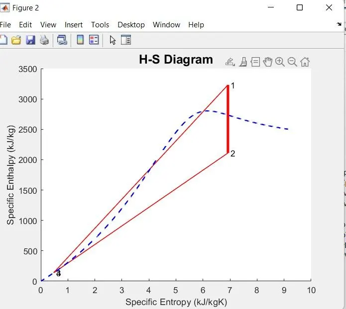
The h-s diagram is showing the relationship between specific enthalpy and specific entropy. This diagram is showing the relation at all stages of the Rankine cycle.

Conclusion:

We have developed a Rankine cycle simulator using MATLAB and also learn about the thermodynamic relationships of the Rankine simulator clearly.

Reference:

YouTube links:

Project 2 - Rankine cycle Simulator

Ship work like this
in your own course.

Talk to a career counsellor

Ship work like thisin your own course.

Talk to a career counsellor

Ship work like this
in your own course.