Week 3 - Solving second order ODEs
Aim: To write a MATLAB program that will simulate the pendulum motion by solving the 2nd order ODE. Also, create an animation of the pendulum's motion.
Solution:
A simple pendulum:
A pendulum is an object hung from a fixed point that swings back and forth under the action of gravity. When a pendulum is displaced sideways from its resting, equilibrium position, it is subject to a restoring force due to gravity that will accelerate it back toward the equilibrium position. The motion of a simple pendulum is very close to Simple Harmonic Motion (SHM). SHM results whenever a restoring force is proportional to the displacement, a relationship often known as Hooke's Law when applied to springs. The period of a pendulum is the time it takes the pendulum to make one full back-and-forth swing.
The equation for the period of a simple pendulum starting at a small angle is: T = 2π√(L/g), with units in seconds. Here, T is the period in seconds (s), π is approximately 3.14, L is the length of the rod or wire in meters and g is the acceleration due to gravity (9.8 m/s²). The reciprocal of this period will give us the frequency of the simple pendulum measured in Hertz. (Quora. (n.d.)).
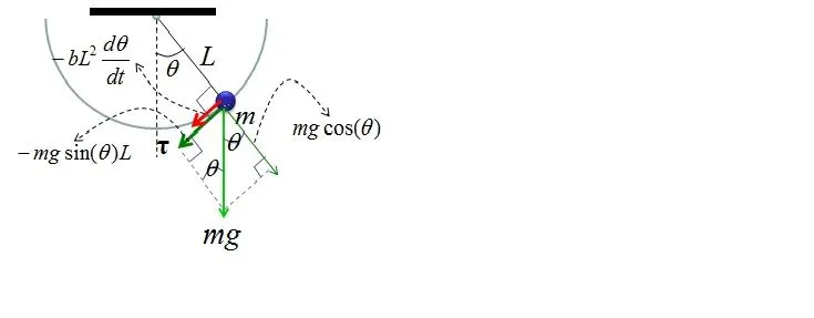
Fig 1 Simple Pendulum
Newton's 2nd Law of Motion governs a simple pendulum. When the law is applied to the pendulum's motion, we obtain a 2nd order ordinary differential equation (ODE) wrt time.
The ODE representing the motion of a simple pendulum (with damping) is given as:
`(d^2 theta) / dt^2 + b/m*(d theta)/dt + g/L*sin theta = 0`.....................................Eqn. 1
Let's consider `theta = theta_1`, then,
`(d theta)/dt = (d theta_1)/dt = theta_2`.............................................................................Eqn. 2
or, `(d^2 theta)/dt^2 = (d^2 theta_1)/dt^2 = d/dt((d theta_1)/(dt)) = (d theta_2)/dt`.........................Eqn. 3
Now, by substituting Eqn. 2 & 3 in Eqn. 1, we get:
`(d^2 theta_1) / dt^2 + b/m*(d theta_1)/dt + g/L*sin theta_1 = 0`
or, `(d theta^2)/dt + b/m*theta_2 + g/L*sin theta_1 = 0`
or, `(d theta^2)/dt = -b/m*theta_2 -g/L*sin theta_1`................................................Eqn. 4
Representing the ODE in matrix form, from Eqn. 3 & 4, we derive:-
`d/dt[(theta_1),(theta_2)] = [(theta_2) , (-b/m*theta_2 -g/L*sin theta_1)]`
Methodology:
1. All the input values are substituted as given in the question.
2. The ODE function is solved and the result is plotted.
3. A separate function is called into the main function in order to solve the ODE.
4. To animate the motion of the pendulum, for loop is used and a video file is generated.
5. The obtained results are displayed.
MATLAB code for solving the ODE and to animate it:
% A program to simulate the pendulum motion & create an animation of it.

clear all
close all
clc

% Input variables
b = 0.05;                             % b = damping coefficient,
g = 9.81;                             % g = gravity in m/s^2,
L = 1;                                % L = length of the pendulum in m,
m = 1;                                % m = mass of the ball in kg.

% Initial condition
theta_0 = [0;3];                      % displacement;angular velocity.

% time points
t_value = linspace(0,20,300);

% Solving the ODE
[t, results] = ode45(@(t,theta) ode_func(t,theta,b,g,L,m),t_value,theta_0);

% plotting

figure(1)

plot(t,results(:,1),'LineWidth',2,'LineStyle','-.', 'Color','r')
hold ON
plot(t,results(:,2),'LineWidth',1,'Color', 'b')

title('SHM of a Simple Pendulum')
legend('Displacement', 'Angular velocity')
xlabel('Time in sec')
ylabel('Plot')
grid ON
hold off

% Animating the transient behaviour of a simple pendulum

% For loop

ct = 1;                             % individual frame

for i = 1:length(results(:,1))

% Initial Cordinates
Xo = 0;
Yo = 0;

% Final Cordinates
X_1 = L*sin(results(i,1));
Y_1 = -L*cos(results(i,1));

% Plotting
figure(2)

plot ([-.5 .5], [0 0], 'linewidth', 10 , 'Color','black');
hold ON
line ([Xo X_1], [Yo Y_1],'linewidth',3, 'color', 'black');
hold ON
plot (X_1,Y_1, 'Marker','o', 'MarkerEdgeColor','r', 'MarkerFaceColor', 'r', 'MarkerSize',25);
title('Motion of a Simple Pendulum')
grid ON


axis([-2 2 -2 2]);                  % Assigning the axis
pause(.03);                         % holds the execution temporarily for the specified time period

hold OFF
M(ct) = getframe(gcf);              % saving the figure window in an array named M
ct = ct+1;                          % each time, incrementing the individual frame by 1

end

movie(M);                           % generates a movie using all the frames

videofile = VideoWriter('The transient behaviour of a Simple Pendulum.AVI','Uncompressed AVI');        % creates a video file
open(videofile);                    % opens the video file
writeVideo(videofile,M);            % writes the captured frames to the video file
close(videofile);                   % closes the video file
The function code:
% the ode function program

function [dtheta_dt] = ode_func(t,theta,b,g,L,m)

theta1 = theta(1);
theta2 = theta(2);

dtheta1_dt = theta2;
dtheta2_dt = -(b/m)*theta2 - (g/L)*sin(theta1);
dtheta_dt =[dtheta1_dt;dtheta2_dt];

end
Errors occurred during coding:
The following error with an incomplete plot was obtained while running the code.
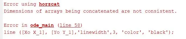
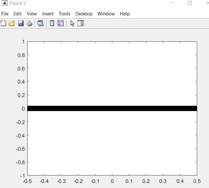
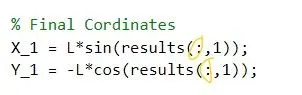
Took me a while to figure out the error, which was a typo actually. Wrong inputs caused the error as highlighted in the picture below. Instead of 'results(i,1)', I typed 'results(:,1)' and that caused the above errors. After going through the codes multiple times, I successfully identified the error and rectified it.
Results:
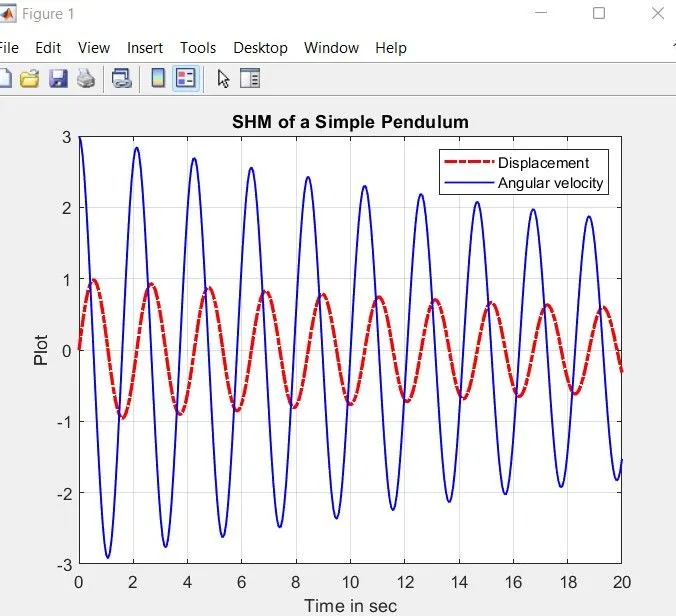
1. The displacement and angular velocity is represented in the following graph:
2. The motion of the pendulum is animated and the link is provided below:
Conclusion:
Thus, a MATLAB program to simulate the transient behaviour of a simple pendulum by solving the 2nd order ODE was successfully executed and the results were obtained.
References
Quora. (n.d.). What is simple pendulum? [online] Available at: https://www.quora.com/What-is-simple-pendulum [Accessed 2 Jun. 2022].