Project 2 - Rankine cycle Simulator
OBJECTIVES:
- To create a Rankine Cycle Simulator using MATLAB and calculate the state points of the Rankine Cycle based on user inputs.
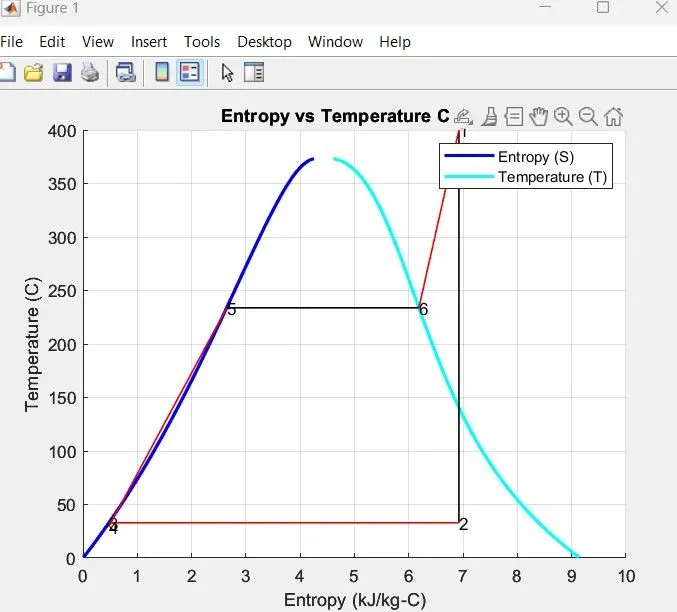
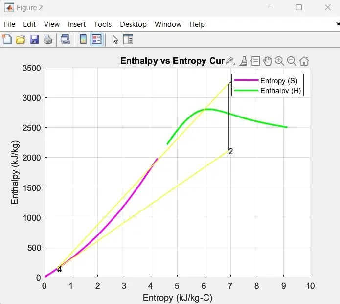
- To plot the corresponding T-S and H-S plots for the given set of inputs.
- To calculate the Net-work and Back work ratio of the Rankine Cycle.
SOLUTION:
Theory of Rankine Cycle:
The Rankine cycle was named after him and describes the performance of steam turbine systems, though the theoretical principle also applies to reciprocating engines such as steam locomotives. In general, the Rankine cycle is an idealized thermodynamic cycle of a constant-pressure heat engine that converts part of heat into mechanical work. In this cycle the heat is supplied externally to a closed loop, which usually uses water (in a liquid and vapor phase) as the working fluid. In contrast to the Brayton cycle, the working fluid in the Rankine cycle undergo the phase change from a liquid to vapor phase and vice versa.
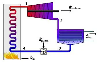
Basic Rankine Cycle Simulator
While many substances could be used as the working fluid in the Rankine cycle (inorganic or even organic), water is usually the fluid of choice due to its favorable properties, such as its non-toxic and unreactive chemistry, abundance, and low cost, as well as its thermodynamic properties. For example, water has the highest specific heat of any common substance – 4.19 kJ/kg K. Moreover it has a very high heat of vaporization, which makes it an effective coolant and medium in thermal power plants and other energy industries. In the case of the Rankine cycle, the Ideal Gas Law almost cannot be used (steam do not follow pV=nRT), therefore all important parameters of water and steam are tabulated in so-called “Steam Tables“.
One of the major advantages of the Rankine cycle is that the compression process in the pump takes place on a liquid. By condensing the working steam to a liquid (inside a condenser) the pressure at the turbine outlet is lowered and the energy required by the feed pump consumes only 1% to 3% of the turbine output power and these factors contribute to higher efficiency for the cycle.
In an ideal Rankine cycle, the system executing the cycle undergoes a series of four processes: two isentropic (reversible adiabatic) processes alternated with two isobaric processes:
- Isentropic compression (compression in centrifugal pumps) – The liquid condensate is compressed adiabatically from state 1 to state 2 by centrifugal pumps (usually by condensate pumps and then by feedwater pumps). The liquid condensate is pumped from the condenser into the higher pressure boiler. In this process, the surroundings do work on the fluid, increasing its enthalpy (h = u+pv) and compressing it (increasing its pressure). On the other hand the entropy remains unchanged. The work required for the compressor is given by WPumps = H2 – H1.
- Isobaric heat addition (in a heat exchanger – boiler) – In this phase (between state 2 and state 3) there is a constant-pressure heat transfer to the liquid condensate from an external source, since the chamber is open to flow in and out. The feedwater (secondary circuit) is heated from to the boiling point (2 → 3a) of that fluid and then evaporated in the boiler (3a → 3). The net heat added is given by Qadd = H3 – H2
- Isentropic expansion (expansion in a steam turbine) – Steam from the boiler expands adiabatically from state 3 to state 4 in a steam turbine to produce work and then is discharged to the condenser (partially condensed). The steam does work on the surroundings (blades of the turbine) and loses an amount of enthalpy equal to the work that leaves the system. The work done by turbine is given by WT = H4 – H3. Again the entropy remains unchanged.
- Isobaric heat rejection (in a heat exchanger) – In this phase the cycle completes by a constant-pressure process in which heat is rejected from the partially condensed steam. There is heat transfer from the vapor to cooling water flowing in a cooling circuit. The vapor condenses and the temperature of the cooling water increases. The net heat rejected is given by Qre = H4 – H1
During a Rankine cycle, work is done on the fluid by the pumps between states 1 and 2 (isentropic compression). Work is done by the fluid in the turbine between stages 3 and 4 (isentropic expansion). The difference between the work done by the fluid and the work done on the fluid is the net work produced by the cycle and it corresponds to the area enclosed by the cycle curve (in pV diagram). The working fluid in a Rankine cycle follows a closed loop and is reused constantly.
As can be seen, it is convenient to use enthalpy and the first law in terms of enthalpy in the analysis of this thermodynamic cycle. This form of the law simplifies the description of energy transfer. At constant pressure, the enthalpy change equals the energy transferred from the environment through heating:
Isobaric process (Vdp = 0):
dH = dQ → Q = H2 – H1
At constant entropy, i.e. in an isentropic process, the enthalpy change equals the flow process work done on or by the system:
Isentropic process (dQ = 0):
dH = Vdp → W = H2 – H1
Isentropic Process
An isentropic process is a thermodynamic process, in which the entropy of the fluid or gas remains constant. It means the isentropic process is a special case of an adiabatic process in which there is no transfer of heat or matter. It is a reversible adiabatic process. The assumption of no heat transfer is very important, since we can use the adiabatic approximation only in very rapid processes.
Isentropic Process and the First Law
For a closed system, we can write the first law of thermodynamics in terms of enthalpy:
dH = dQ + Vdp
or
dH = TdS + Vdp
Isentropic process (dQ = 0):
dH = Vdp → W = H2 – H1
Isobaric Process
An isobaric process is a thermodynamic process, in which the pressure of the system remains constant (p = const). The heat transfer into or out of the system does work, but also changes the internal energy of the system.
Since there are changes in internal energy (dU) and changes in system volume (∆V), engineers often use the enthalpy of the system, which is defined as:
H = U + pV
Isobaric Process and the First Law
The classical form of the first law of thermodynamics is the following equation:
dU = dQ – dW
In this equation dW is equal to dW = pdV and is known as the boundary work. In an isobaric process and the ideal gas, part of heat added to the system will be used to do work and part of heat added will increase the internal energy (increase the temperature). Therefore it is convenient to use the enthalpy instead of the internal energy.
Isobaric process (Vdp = 0):
dH = dQ → Q = H2– H1
At constant entropy, i.e. in isentropic process, the enthalpy change equals the flow process work done on or by the system.
Thermal Efficiency of Rankine Cycle
In general the thermal efficiency, ηth, of any heat engine is defined as the ratio of the work it does, W, to the heat input at the high temperature, QH.
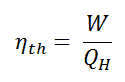
The thermal efficiency, ηth, represents the fraction of heat, QH, that is converted to work. Since energy is conserved according to the first law of thermodynamics and energy cannot be be converted to work completely, the heat input, QH, must equal the work done, W, plus the heat that must be dissipated as waste heat QC into the environment. Therefore we can rewrite the formula for thermal efficiency as:
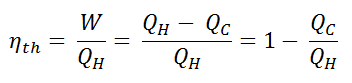
This is very useful formula, but here we express the thermal efficiency using the first law in terms of enthalpy.
Typically most of nuclear power plants operate multi-stage condensing steam turbines. In these turbines, the high-pressure stage receives steam (this steam is nearly saturated steam – x = 0.995 – point C at the figure; 6 MPa; 275.6°C) from a steam generator and exhaust it to moisture separator-reheater (point D). The steam must be reheated in order to avoid damages that could be caused to blades of steam turbine by low quality steam. The reheater heats the steam (point D) and then the steam is directed to the low-pressure stage of steam turbine, where expands (point E to F). The exhausted steam then condenses in the condenser and it is at a pressure well below atmospheric (absolute pressure of 0.008 MPa), and is in a partially condensed state (point F), typically of a quality near 90%.
In this case, steam generators, steam turbine, condensers and feedwater pumps constitute a heat engine, that is subject to the efficiency limitations imposed by the second law of thermodynamics. In ideal case (no friction, reversible processes, perfect design), this heat engine would have a Carnot efficiency of
= 1 – Tcold/Thot = 1 – 315/549 = 42.6%
where the temperature of the hot reservoir is 275.6°C (548.7K), the temperature of the cold reservoir is 41.5°C (314.7K). But the nuclear power plant is the real heat engine, in which thermodynamic processes are somehow irreversible. They are not done infinitely slowly. In real devices (such as turbines, pumps, and compressors) a mechanical friction and heat losses cause further efficiency losses.
To calculate the thermal efficiency of the simplest Rankine cycle (without reheating) engineers use the first law of thermodynamics in terms of enthalpy rather than in terms of internal energy.
The first law in terms of enthalpy is:
dH = dQ + Vdp
In this equation the term Vdp is a flow process work. This work, Vdp, is used for open flow systems like a turbine or a pump in which there is a “dp”, i.e. change in pressure. There are no changes in control volume. As can be seen, this form of the law simplifies the description of energy transfer. At constant pressure, the enthalpy change equals the energy transferred from the environment through heating:
Isobaric process (Vdp = 0):
dH = dQ → Q = H2 – H1
At constant entropy, i.e. in isentropic process, the enthalpy change equals the flow process work done on or by the system:
Isentropic process (dQ = 0):
dH = Vdp → W = H2 – H1
It is obvious, it will be very useful in analysis of both thermodynamic cycles used in power engineering, i.e. in Brayton cycle and Rankine cycle.
The enthalpy can be made into an intensive, or specific, variable by dividing by the mass. Engineers use the specific enthalpy in thermodynamic analysis more than the enthalpy itself. It is tabulated in the steam tables along with specific volume and specific internal energy. The thermal efficiency of such simple Rankine cycle and in terms of specific enthalpies would be:

It is very simple equation and for determination of the thermal efficiency you can use data from steam tables.
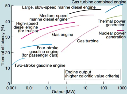
In modern nuclear power plants the overall thermal efficiency is about one-third (33%), so 3000 MWth of thermal power from the fission reaction is needed to generate 1000 MWe of electrical power. The reason lies in relatively low steam temperature (6 MPa; 275.6°C). Higher efficiencies can be attained by increasing the temperature of the steam. But this requires an increase in pressures inside boilers or steam generators. However, metallurgical considerations place an upper limits on such pressures. In comparison to other energy sources the thermal efficiency of 33% is not much. But it must be noted that nuclear power plants are much more complex than fossil fuel power plants and it is much easier to burn fossil fuel ,than to generate energy from nuclear fuel. Sub-critical fossil fuel power plants, that are operated under critical pressure (i.e. lower than 22.1 MPa), can achieve 36–40% efficiency.
MATLAB CODE:
clear all
close all
clc

% DISPLAYING THE CONTENT
fprintf("\n                              RANKINE CYCLE SIMULATOR                            \n");
fprintf("\n Process 1-2 : Isentropic expansion in the Turbine \n");
fprintf("\n Process 2-3 : Isobaric heat rejection by the Condenser \n");
fprintf("\n Process 3-4 : Isentropic compression in the Pump \n");
fprintf("\n Process 4-1 : Isobaric heat addition by the Boiler \n");

% USER INPUTS
t1 = input('\n Enter the Temperature at the Turbine inlet (in Celsius) = ');
p1 = input('\n Enter the Pressure at the Turbine inlet (in bar) = ');
p2 = input('\n Enter the Turbine Outlet Pressure or Condenser Inlet Pressure(in bar) = ');

% TURBINE INLET PARAMETERS
tsat_1 = XSteam('Tsat_p',p1);
if t1 > tsat_1
    h1 = XSteam('h_pt',p1,t1);
    s1 = XSteam('s_pt',p1,t1);
elseif t1 == tsat_1
        h1 = XSteam('hV_p',p1);
        s1 = XSteam('sV_p',p1);
    else
        fprintf("\n Enter higher value of Turbine inlet temperature (in Celsius)!!! \n\n");
end


% TURBINE OUTLET CONDITIONS

s2 = s1;                        %isentropic expansion in the turbine
ssat_2 = XSteam('sV_p',p2);
if s2 < ssat_2
    sf_2 = XSteam('sL_p',p2);
    sg_2 = XSteam('sV_p',p2);

% x = the dryness fraction of the steam
    x = (s2 - sf_2)/(sg_2 - sf_2);
    hf_2 = XSteam('hL_p',p2);
    hg_2 = XSteam('hV_p',p2);
    h2  = hf_2 + x*(hg_2 - hf_2);
    t2 = XSteam('Tsat_p',p2);
else
    x = 1;
    h2 = XSteam('hV_p',p2);
    t2 = XSteam('Tsat_p',p2);
end


% PUMP INLET CONDITIONS
p3 = p2;
t3 = XSteam('Tsat_p',p3);
h3 = XSteam('hL_p',p3);
s3 = XSteam('sL_p',p3);
v3 = XSteam('vL_p',p3);


% BOILER INLET CONDITIONS
p4 = p1;
s4 = s3;
v4 = XSteam('v_ps',p4,s4);
cp4 = XSteam('Cp_ps',p4,s4);
cv4 = XSteam('Cv_ps',p4,s4);
gamma = cp4/cv4;
G = (gamma - 1)/gamma;
t4 = t3*(p2/p1)^G;

% WORK REQUIRED BY THE PUMP
W_p = v3*(p4 - p3)*100;

% W_p = h4 - h3
h4 = W_p + h3;


% CONDITIONS AT STATE 5 AND STATE 6 IN (4-1) STAGE
t5 = XSteam('Tsat_p',p4);
s5 = XSteam('sL_p',p4);
t6 = t5;
s6 = XSteam('sV_p',p4);


% WORK DONE BY THE TURBINE
W_t = h1 - h2;

% HEAT INPUT
Q_in = h1 - h4;

% HEAT OUTPUT
Q_out = h2 - h3;

% NET-WORK OBTAINED
W_net = W_t - W_p;

% Efficiency of the Rankine Cycle
efficiency = (W_net*100)/Q_in;

% BACK WORK RATIO
W_ratio = W_p/W_t;

% SPECIFIC STEAM COSUMPTION
Steam_consumption = 3600/W_net;


%DISPLAYING THE OBTAINED INFORMATION
fprintf("\n  <----------------------RESULTS----------------------->  \n");
fprintf("At State Point 1:                              At State Point 4: \n P1 = %4.2f bar                                 P4 = %4.2f bar \n T1 = %.2f C                                  T4 = %4.2f C  \n H1 = %.2f kJ/kg                             H4 = %4.2f kJ/kg  \n S1 = %4.2f kJ/kg-C                              S4 = %4.2f kJ/kg-C \n",p1,p4,t1,t4,h1,h4,s1,s4);
fprintf("\nAt State Point 2:                              At State Point 3: \n P2 = %4.2f bar                                  P3 = %4.2f bar \n T2 = %.2f C                                   T3 = %4.2f C  \n H2 = %.2f kJ/kg                             H3 = %4.2f kJ/kg  \n S2 = %4.2f kJ/kg-C                              S3 = %4.2f kJ/kg-C \n",p2,p3,t2,t3,h2,h3,s2,s3);

fprintf("\n Work required by the pump in the Rankine Cycle = %2.2f kJ/kg\n",W_p);
fprintf("\n Work produced by the turbine in the Rankine Cycle = %2.2f kJ/kg\n",W_t);
fprintf("\n Net Work obtained in the Rankine Cycle = %2.2f kJ/kg\n",W_net);
fprintf("\n Heat input to the Rankine Cycle = %2.2f kJ/kg\n",Q_in);
fprintf("\n The efficiency of the Rankine Cycle = %2.2f \n",efficiency);
fprintf("\n Back Work Ratio in the Rankine Cycle = %.7f \n",W_ratio);
fprintf("\n Specific Steam Consumption in the Rankine Cycle = %2.2f kg/kWh \n",Steam_consumption);


% PLOTS

% T-S DIAGRAM
T = linspace(0,373.946,500);      % critical point of water occurs at 373.946 degree Celsius
figure(1);
hold on
for i = 1 : length(T)
    s_l(i) = XSteam('sL_T',T(i));
    s_g(i) = XSteam('sV_T',T(i));
    h_l(i) = XSteam('hL_T',T(i));
    h_g(i) = XSteam('hV_T',T(i));
end

plot(s_l,T,'linewidth',2,'color','b');
plot(s_g,T,'linewidth',2,'color','c');
plot([s1 s2],[t1 t2],'linewidth',1,'color','k');
text(s1,t1,'1');
plot([s2 s3],[t2 t3],'linewidth',1,'color','r');
text(s2,t2,'2');
plot([s3 s4],[t3 t4],'linewidth',1,'color','k');
text(s3,t3,'3');
plot([s4 s5],[t4 t5],'linewidth',1,'color','r');
text(s4,t4,'4');
plot([s5 s6],[t5 t6],'linewidth',1,'color','k');
text(s5,t5,'5');
plot([s6 s1],[t6 t1],'linewidth',1,'color','r');
text(s6,t6,'6');
xlabel('Entropy (kJ/kg-C)');
ylabel('Temperature (C)');
title('Entropy vs Temperature Curve');
legend('Entropy (S)','Temperature (T)');
grid on
hold off


% H-S DIAGRAM
figure(2);
hold on
plot(s_l,h_l,'linewidth',2,'color','m');
plot(s_g,h_g,'linewidth',2,'color','g');
plot([s1 s2],[h1 h2],'linewidth',1,'color','k');
text(s1,h1,'1');
plot([s2 s3],[h2 h3],'linewidth',1,'color','y');
text(s2,h2,'2');
plot([s3 s4],[h3 h4],'linewidth',1,'color','k');
text(s3,h3,'3');
plot([s4 s1],[h4 h1],'linewidth',1,'color','y');
text(s4,h4,'4');
xlabel('Entropy (kJ/kg-C)');
ylabel('Enthalpy (kJ/kg)');
title('Enthalpy vs Entropy Curve');
legend('Entropy (S)','Enthalpy (H)');
grid on
CODE EXPLANATION:
- The code begins by displaying the various processes involved in the Rankine cycle, including the isentropic expansion in the turbine, the isobaric heat rejection by the condenser, the isentropic compression in the pump, and the isobaric heat addition by the boiler.
- Then the code takes user inputs for the temperature and pressure at the turbine inlet, as well as the turbine outlet pressure or condenser inlet pressure.
- The code then calculates the various state points and parameters of the cycle, such as the enthalpy, entropy, and temperature at each state, as well as the work done by the turbine and the pump, and the efficiency and back work ratio of the cycle.
- The code makes use of the XSteam library, which provides a set of functions for calculating the thermodynamic properties of water and steam. The XSteam library is not a built-in library in MATLAB, so it must be downloaded and installed separately.
- The code then displays the results of the calculations, including the thermodynamic properties at each state point, the work done by the pump and the turbine, and the efficiency and back work ratio of the cycle.
- Finally, the T-S & H-S graphs are plotted and displayed.
OUTPUT:
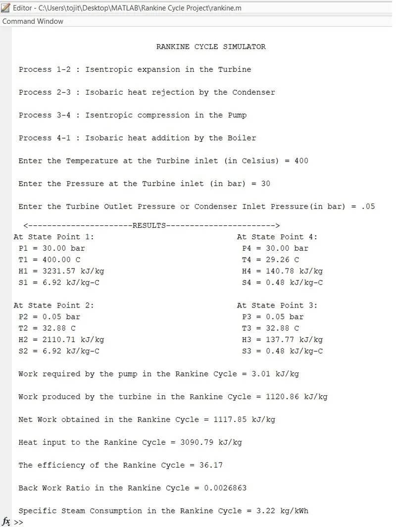
The Net-work of the Rankine Cycle = 1117.85 kJ/kg
The Back work ratio of the Rankine Cycle = 0.0026863.
T-S graph:
H-S graph:
No major errors occurred during coding.
REFERENCES:
Thermal Engineering. 2023. What is Theory of Rankine Cycle - Equations and Calculation - Definition. [ONLINE] Available at: https://www.thermal-engineering.org/what-is-theory-of-rankine-cycle-equations-and-calculation-definition/. [Accessed 05 March 2023].