Challenge

Project 1 - Parsing NASA thermodynamic data

TToji Thomas24 Feb 2023

OBJECTIVES:

1. To write a MATLAB code to extract the 14 coefficients and calculate the Enthalpy (H), Entropy (S), and Specific Heat (Cp) for all the species in the given data file ("THERMO.dat").

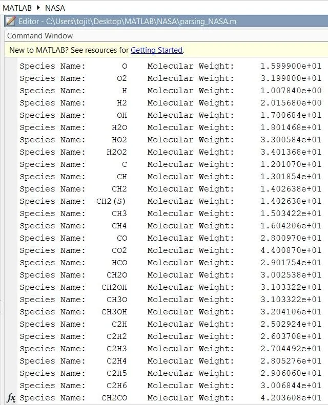
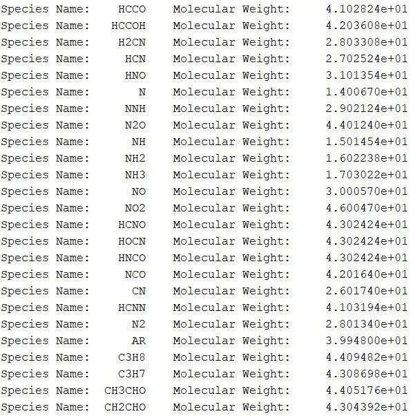
2. Calculate the Molecular Weight of each species and display it in the command window.

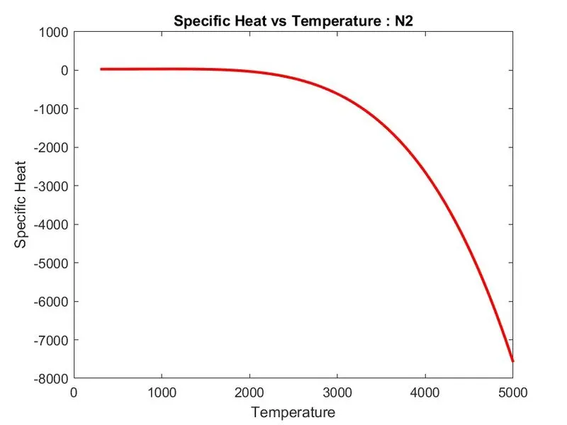
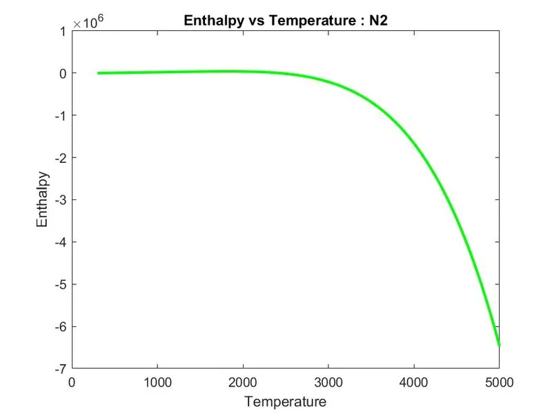
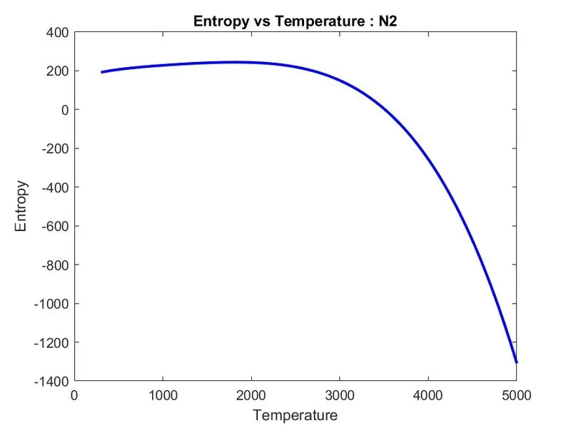
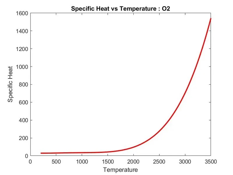
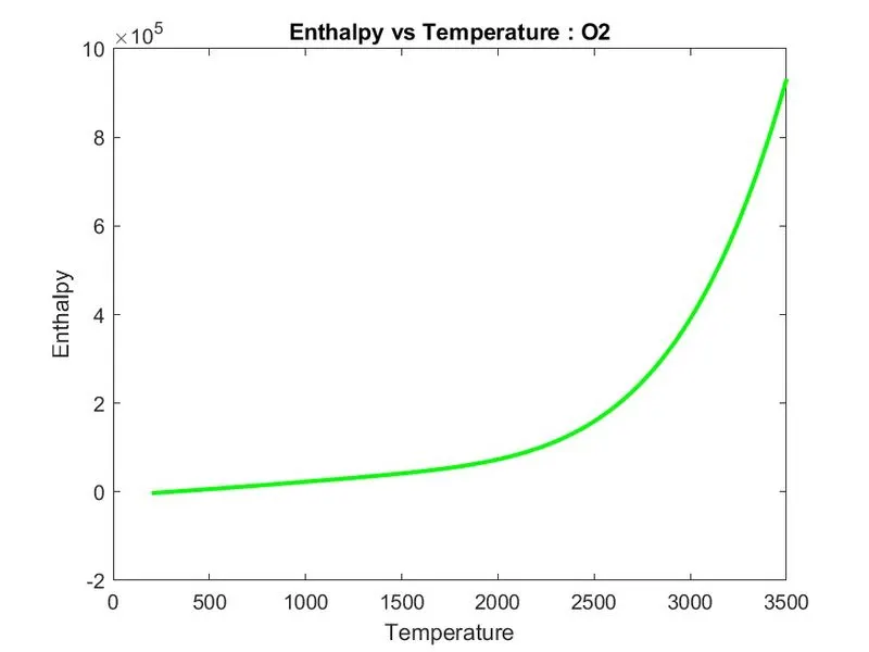
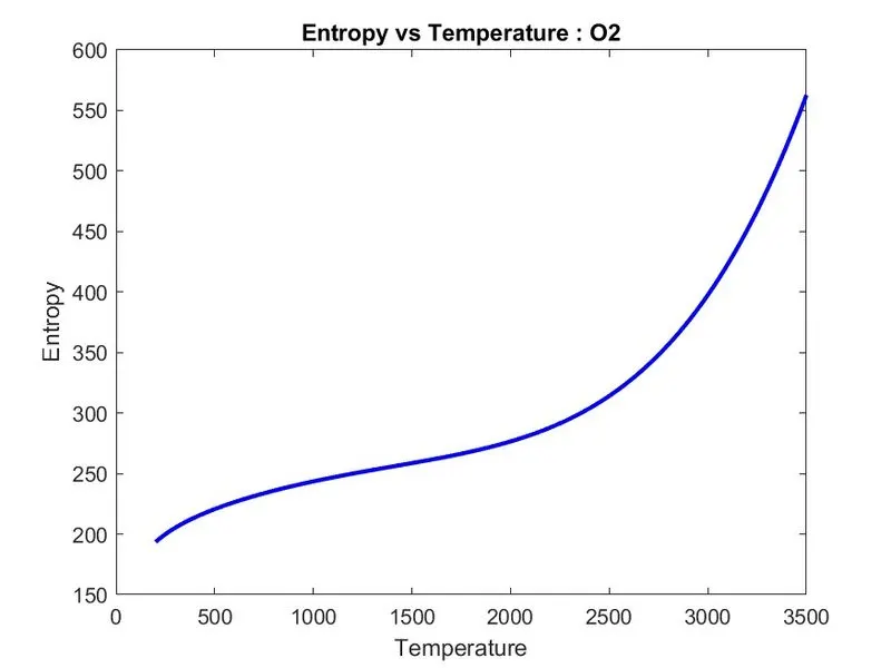
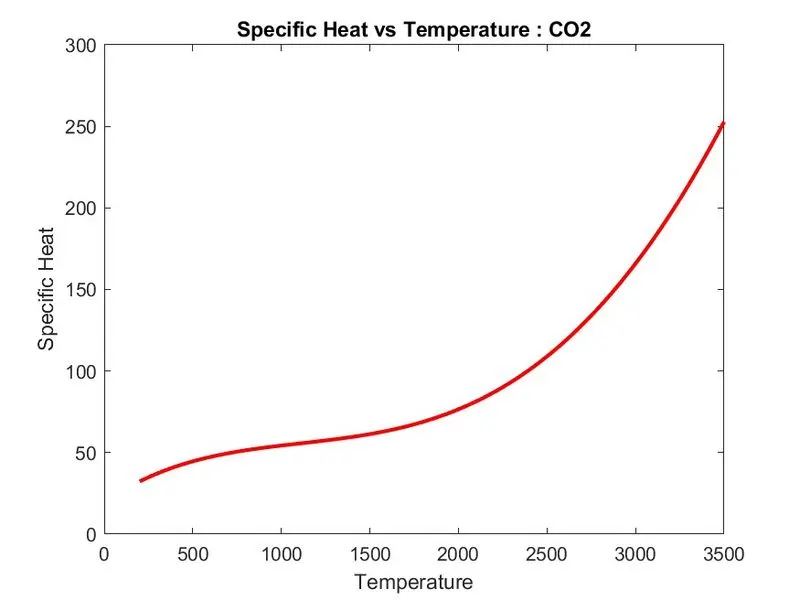
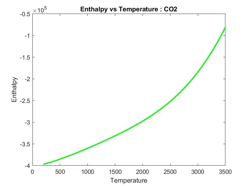
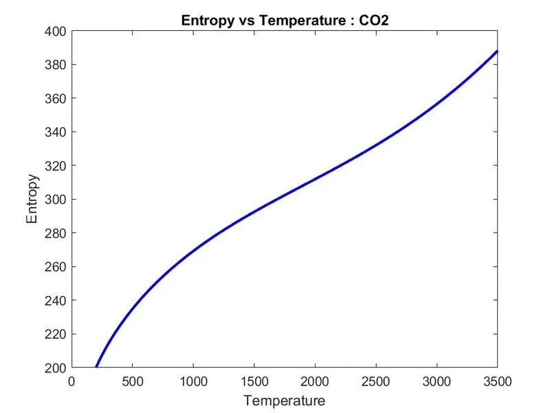
3. Plot the Cp, H, and S for the local temperature range (low temperature: high temperature) specific for each species.

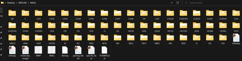
4. Save the plots as images with appropriate names and dump them in separate folders for each species with a suitable name. All these should be generated automatically.

Attachments needed:

Screenshot of the window where all the folders are saved.
Plots for O2, N2, and CO2 species.

SOLUTION:

Parsing in MATLAB refers to the process of analyzing a string of characters or a sequence of tokens to determine its structure or syntax according to a specific set of rules or grammar.

In MATLAB, parsing can be used in a variety of contexts, including:

Command-line input: MATLAB uses a parser to interpret and execute commands entered at the command prompt.
Function arguments: When a function is called, its input arguments are parsed to ensure that they are valid and conform to the expected data type and format.
File input/output: MATLAB uses parsing to read and write files in various formats, such as CSV, XML, and JSON.
Script files: MATLAB scripts are parsed by the interpreter before execution to ensure that they are syntactically correct and to resolve any variables and functions used in the script.

In summary, parsing in MATLAB is the process of analyzing and interpreting input data to ensure that it conforms to a specific syntax or grammar. This is an essential part of many MATLAB operations and is used in a variety of contexts, including command-line input, function arguments, file input/output, and script files.

Given Formula:

Here R is the universal gas constant,

T is the temperature,

Cp is the Specific Heat,

H is the Enthalpy,

S is the Entropy.

MAIN MATLAB CODE:

clear all
close all
clc

% Read the Data file
f1 = fopen('THERMO.dat','r');

% Read the first line of the data file
Header = fgetl(f1);

% Read the second line of the data file
overall_global_temp = fgetl(f1);

% Calculate Global Temperatures
temp = strsplit(overall_global_temp,' ');
global_minimum = str2num(temp{2});
global_mid = str2num(temp{3});
global_maximum = str2num(temp{4});

% Skipping the next 3 lines
for i = 1:3
    skip = fgetl(f1);
end


% Creating a loop to go through all 53 species of data
for j = 1:53
    main_line = fgetl(f1);
    species_data = strsplit(main_line,' ');
    
   % Calculate Local Temperatures
    local_minimum = str2num(species_data{end-3});
    local_mid = str2num(species_data{end-1});
    local_maximum = str2num(species_data{end-2});
    T = linspace(local_minimum, local_maximum, 500);
    
    species_name = species_data{1};

    % Reading 3 lines containing seven high temp & low temp coefficients
    line_1 = fgetl(f1);
    line_2 = fgetl(f1);
    line_3 = fgetl(f1);
    
    % Finding position of 'E'
    x = strfind(line_1,'E');
    y = strfind(line_2,'E');
    z = strfind(line_3,'E');
    
    % Temperature coefficients_High
    a1 = str2num(line_1(1:x(1)+3));
    a2 = str2num(line_1(x(1)+4:x(2)+3));
    a3 = str2num(line_1(x(2)+4:x(3)+3));
    a4 = str2num(line_1(x(3)+4:x(4)+3));
    a5 = str2num(line_1(x(4)+4:x(5)+3));
    a6 = str2num(line_2(1:y(1)+3));
    a7 = str2num(line_2(y(1)+4:y(2)+3));
    
    % Temperature coefficients_Low
    b1 = str2num(line_2(y(2)+4:y(3)+3));
    b2 = str2num(line_2(y(3)+4:y(4)+3));
    b3 = str2num(line_2(y(4)+4:y(5)+3));
    b4 = str2num(line_3(1:z(1)+3));
    b5 = str2num(line_3(z(1)+4:z(2)+3));
    b6 = str2num(line_3(z(2)+4:z(3)+3));
    b7 = str2num(line_3(z(3)+4:z(4)+3));
    
    
    % Universal Gas Constant (R)
    R = 8.314;

    % Calculating Molecular Weight (MW)
    [MW_j] = molecular_weight(species_name);


    % Calculating Specific Heat (Cp)
    [Cp] = specific_heat(a1,a2,a3,a4,a5,b1,b2,b3,b4,b5,R,T,local_mid);
    
    % Calculating Enthalpy (H)
    [H] = enthalpy(a1,a2,a3,a4,a5,a6,b1,b2,b3,b4,b5,b6,R,T,local_mid);
    
    % Calculating Entropy (S)
    [S] = entropy(a1,a2,a3,a4,a5,a7,b1,b2,b3,b4,b5,b7,R,T,local_mid);
    
    
  
    % Plots
    set(0,'DefaultFigureVisible','off')
    m(1)=figure;
    plot(T, Cp, 'linewidth',2,'color','r')
    xlabel('Temperature')
    ylabel('Specific Heat')
    title(['Specific Heat vs Temperature : ',species_name])
    
    m(2)=figure;
    plot(T, H, 'linewidth',2,'color','g')
    xlabel('Temperature')
    ylabel('Enthalpy')
    title(['Enthalpy vs Temperature : ',species_name])
    
    m(3)=figure;
    plot(T, S, 'linewidth',2,'color','b')
    xlabel('Temperature')
    ylabel('Entropy')
    title(['Entropy vs Temperature : ',species_name])
    
    
    % Displaying Molecular Weight of all species
    fprintf('Species Name: %7s    ',species_name)
    fprintf('Molecular Weight: %16s \n', MW_j)

    % Saving species names to a specific folder
    cd('C:\Users\tojit\Desktop\MATLAB\NASA')
    mkdir(species_name);
    cd(species_name);
    
    % Saving the plots as images (.jpg)
    saveas(m(1),'Cp_vs_Temperature.jpg')
    saveas(m(2),'H_vs_Temperature.jpg')
    saveas(m(3),'S_vs_Temperature.jpg')
    

    % Saving the rest of the data
    f2 = fopen('data_parsing_NASA.txt','w');
    fprintf (f2, '%10s : %10s \n','Species Name',species_name);
    fprintf (f2, '%10s : %10.5s \n','Molecular Weight',MW_j);
    fprintf (f2, 'For Local Temperature range : %4.2fk to %4.2fk \n',local_minimum,local_maximum);
    fprintf (f2, '%5s %5s %15s %15s \n','Temperature', 'Specific Heat', 'Enthalpy', 'Entropy');
    fprintf (f2, '%10.2f %16.2f %18.2f %20.2f \n', T, Cp, H, S); 
    
    cd('C:\Users\tojit\Desktop\MATLAB\NASA');
end

CODE EXPLANATION:

The program starts by clearing all previous values and opening the 'THERMO.dat' file using the fopen command.
The fgetl command is used to read the next line, which is the header of the file.
The following line gives the global temperature range, which is split into minimum, middle, and maximum values using strsplit and str2num commands.
The next three lines are unnecessary and are ignored using a for loop.
A loop is used to extract coefficients and calculate thermodynamic properties for 53 species by using the fgetl, strsplit, and str2num commands.
The local minimum, middle, and maximum temperatures are found for each species, and T values are obtained using the linspace command.
The high and low-temperature coefficients (a1-a7, b1-b7) are extracted using the str2num command, and the universal gas constant (R) is set to 8.314.
The thermodynamic properties of the species are calculated using Cp, H, S, and MW_j functions.
The program plots Specific Heat, Enthalpy, and Entropy vs. Temperature for all the species, and the set command is used to avoid random opening of plot windows.
The fprintf command is used to print molecular weight data in the command window with input arrays for species name and MW_j.
The species name data is saved using the mkdir and cd commands, and plots for the respective species are saved in .jpg format using the saveas command.
The program writes test data to the 'data_parsing_NASA.txt' file using the fopen command, and the data string and desired spacing are specified.
The cd command is used to return to the original file location to complete the loop.

a. Code to calculate Molecular Weight:

% Molecular Weight Function_MW

function [MW] = molecular_weight(species_name)
elements = ['H', 'C', 'N', 'O', 'Ar'];

atomic_weight = [1.00784, 12.0107, 14.0067, 15.999, 39.948];

MW = 0; 

for i = 1:length(species_name)
    for j = 1:length(elements)
        
        if strcmp(species_name(i),elements(j))==1
           MW = atomic_weight(j) + MW;
           atomicweight = atomic_weight(j);
           end
    end
    
    n = str2num(species_name(i));
    
    if n>1
       MW = atomicweight*(n-1) + MW;
    end
    
end
end

Explanation:

The fumction command for determining molecular weight is established.
The function takes the species name as an input and creates a string array with elements that represent the atomic symbols of Hydrogen, Carbon, Nitrogen, Oxygen, and Argon, each with their corresponding atomic weight.
The initial molecular weight is set to zero.
The code then uses a 'for loop' and the 'strmcp' command to compare the species name with each element in the string array.
When the species name matches an element in the array, the code calculates the atomic weight by subtracting the old atomic weight from the current species' atomic weight.
The atomic weight is multiplied by (n-1), where 'n' is the number of atoms of that type in the molecule.
Finally, the atomic weights are summed up to calculate the molecular weight of the species.

b. Code to calculate Specific Heat:

% Specific Heat Function_Cp/R

function [Cp] = specific_heat(a1,a2,a3,a4,a5,b1,b2,b3,b4,b5,R,T,local_mid)

if T<=local_mid
    Cp = R*(a1 + (a2.*T) + (a3.*(T.^2)) + (a4.*(T.^3)) + (a5.*(T.^4)));
else
    Cp = R*(b1 + (b2.*T) + (b3.*(T.^2)) + (b4.*(T.^3)) + (b5.*(T.^4)));
end

Explanation:

Function command is established for Cp with inputs of low & high temperature coefficients, Universal gas constant (R), Temperature (T) and local mid temperature.
Then 'if else' command is used to check the condition whether T is <= to local mid temperature.
Depending on this condition, the Cp is calculated using both low and high temperature coefficients.

c. Code to calculate Enthalpy:

% Enthalpy Function_H

function [H] = enthalpy(a1,a2,a3,a4,a5,a6,b1,b2,b3,b4,b5,b6,R,T,local_mid)

if T<= local_mid
    H = R.*T.*(a1 + (a2.*(T)./(2)) + (a3.*((T).^2)./(3)) + (a4.*((T).^3)./(4)) + (a5.*((T).^4)./(5)) + (a6)./(T));
else
    H = R.*T.*(b1 + (b2.*(T)./(2)) + (b3.*((T).^2)./(3)) + (b4.*((T).^3)./(4)) + (b5.*((T).^4)./(5)) + (b6)./(T));
end

Explanation:

Function command is established for H with inputs of low & high temperature coefficients, Universal gas constant (R), Temperature (T) and local mid temperature.
Then 'if else' command is used to check the condition whether T is <= to local mid temperature.
Low temperature coefficent a6 & High temperature coefficient b6 is calculated additionally.
Enthalpy (H) is then calculated.

d. Code to calculate Entropy:

% Entropy Function_S

function [S] = entropy(a1,a2,a3,a4,a5,a7,b1,b2,b3,b4,b5,b7,R,T,local_mid)
if T<= local_mid
    S = R*((a1.*(log(T))) + (a2.*(T)) + (a3.*((T).^2)./(2)) + (a4.*((T).^3)./(3)) + (a5.*((T).^4)./(4)) + (a7));
else
    S = R*((b1.*(log(T))) + (b2.*(T)) + (b3.*((T).^2)./(2)) + (b4.*((T).^3)./(3)) + (b5.*((T).^4)./(4)) + (b7));
end

Explanation:

Function command is established for S with inputs of low & high temperature coefficients, Universal gas constant (R), Temperature (T) and local mid temperature.
Then 'if else' command is used to check the condition whether T is <= to local mid temperature.
Here a7 & b7 is calculated automatically.
Entropy (S) is then calculated.

RESULT:

Molecular Weight of each species:

Plots for N2:

Plots for O2:

Plots for CO2:

Folders:

CONCLUSION:

Thus, a MATLAB code was successfully written to extract the 14 coefficients from the given data file and the Enthalpy (H), Entropy (S), and Specific Heat (Cp) for all the species in the given data file were successfully calculated.
Plots Cp vs Temperature, H vs Temperature, and S vs Temperature for species N2, O2 & CO2 were displayed.
Also, the Molecular Weight of each species were determined.

No major errors occured during coding. Minor errors were immediately rectified.

Project 1 - Parsing NASA thermodynamic data

Ship work like this
in your own course.

Talk to a career counsellor

Ship work like thisin your own course.

Talk to a career counsellor

Ship work like this
in your own course.