Week 3 - Solving second order ODEs

Objectives :

Write a program that solves the following ODE.

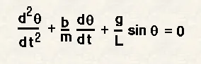
Write a program in Matlab to simulate a pendulum motion.

What is a simple pendulum?

A mechanical system in which oscillatory motion takes place is known as the simple pendulum.

A simple pendulum consists of two main objects which is a thread and a ball.

while solving a pendulum problem the mass of the pendulum ball is considered as M which is the notion of the term mass and the length of the thread is considered as L.

One end of the thread is fixed and the other will be hanging with the ball to attain the oscillatory motion once it is released with kinetic energy.

Solving a second order equation :

In order to use the second order equation in Matlab, we have to convert the second order ODE into a series of first order differential equations. Using a series of the first ODE the equation can be solved or utilised via of the function command.

MATLAB CODING FOR FUNCTION COMMAND:

function [dtheta_dt]= ode_func(t,theta,b,g,l,m)

theta1=theta(1)
theta2=theta(2)
dtheta1_dt = theta2;
dtheta2_dt = -(b/m)*theta2 - (g/l)*sin(theta1);
dtheta_dt= [dtheta1_dt; dtheta2_dt];
end

By solving this equation, Two values will be appeared as a result in a matix form of 2x1.

MATLAB CODING FOR SIMULATE A SIMPLE PENDULUM MOTION:

clc 
clear all
close all

b=0.05;
g=9.81;
l=1;
m=1; 

%Initial condition

theta_0= [0;3];

%Time Points

t_span=linspace(0,20,500);

%solving an ODE
[t, results] = ode45(@(t,theta) ode_func(t,theta,b,g,l,m),t_span,theta_0);


subplot(2,1,1)
plot(t,results(:,1),'b','linewidth',1)
xlabel('time t in sec')
ylabel('Angular displacement')
title('Displacement plot')
legend('Displacement')

hold on
subplot(2,1,2)
plot(t,results(:,2),'r','linewidth',1)
xlabel('Time t in sec')
ylabel('Angular Velocity')
title('Velocity plot')
legend('Velocity')


figure(2)
plot(t,results(:,1),'b','linewidth',1)
xlabel('time t in sec')
ylabel('Angular displacement')
legend('Displacement')

hold on

plot(t,results(:,2),'r','linewidth',1)
xlabel('Time t in sec')
ylabel('Angular Velocity')
title('Time vs displacement and velocity plot')
legend('Displacement','Velocity')


%Animation for simple pendulum

theta2= results(:,1);

ct=1

for i = 1:length(theta2)
    theta = theta2(i);
    x0=0;
    y0=0;
     
    x1= l*cos(3*pi/2+theta);
    y1=l*sin(3*pi/2+theta);

    %ploting the pendulum

    figure(3)

    plot([-1 1] ,[0 0],'color','k')

    hold on 

    plot([x0 x1] ,[y0 y1],'color','r','linewidth',2)

    plot(x1,y1,'o', 'markers',20,"markerfacecolor","k")
    hold off
    grid on
    axis([-2 2 -2 2])

    pause(0.001)

    N(ct)= getframe(gcf);

    ct=ct+1

end

movie(N)

videofile=VideoWriter('Simple_pendulum_video.avi','Uncompressed AVI');

open(videofile)

writeVideo(videofile,N)

close(videofile)

THE PLOT :

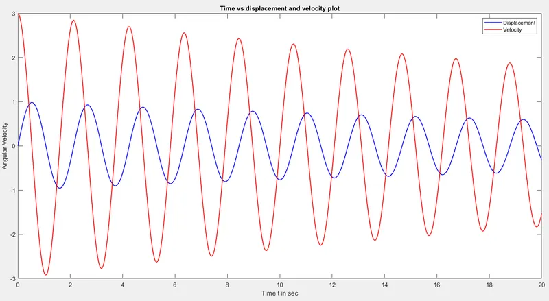
This plot provides a general idea of angular displacement and angular velocity with a respective time and a damping coefficient.

SUBPLOT :

Video link of simple pendulum animation in MatLab:

If this link was not redirecting to youtube, please copy the link and paste it into the youtube search box.

https://youtu.be/gSfsX0XZYXE

In that video, we could get to know how the pendulum moves for the respective parameters.

CODING EXPLANATION :

b = damping coefficient

g = gravitational force

l = length of the thread

m = mass

The theta_0 is an initial condition of the pendulum.

theta_0 = [Initial value of a displacement ; Initial value of a velocity].

T_span = Time taken or time span

ODE45 is an inbuilt command in MatLab which solves only the first Order Differential Equation. In order to utilize this command, we have to convert our given ODE into a series of two first-order differential equations.

Once the ODE45 is derived as a result [t, results] values will be appeared where t is a time and results have two columns which were the values of displacement and velocity for a certain time interval.

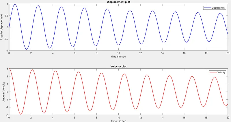
Plotting the three parameters which are t, displacement and velocity will display the plot of the time vs displacement, and the velocity plot which is available above the coding explanation heading.

To create a Pendulum animation we need to use a few commands which is inbuilt in Matlab

for loop is a command which can be used to reuse a particular code, again and again, for certain times.

Here, for loop is used to attain a different position for the pendulum. The length of the thread and angle will be changing each time the for loop command run.

x1 and y1 are the end position of the thread with the bob where the other end is fixed.

Marker command will determine the size of the ball or bob.

o is used to determine the shape of the bob.

Markerfacecolor command will determine the color of the ball or bob.

SYNTAX FOR MAKING AN ANIMATION MOVIE :

N(ct)=getframe(gcf);

Here N is variable

gcf=get current frame

ct=ct+1

Here, I am gradually changing the frame one by one in a single plot and making a video.

movie(N)

M is variable, so the movie will be created according to the position or values of the variable M.

videofile=VideoWriter('FILE_NAME.avi','Uncompressed AVI');

Here, I am creating a file name for the movie and how I want it to be either compressed or uncompressed.

open(videofile)

opening the videofile

writeVideo(videofile,N)

Feeding the N values into a video file by writing the video

close(videofile)

closing the videofile.

APPLICATION OF THIS PROBLEM :

By solving this problem we could get to know what are the positions will this pendulum can achieve. How much damping force is needed to stop the pendulum or slow down.

We can use this problem to test the suspension for a particular damping force or design a suspension that could withstand more shocks by increasing the damping value.

APPLICATION :

Automobile field

Aviation sector

Ports

Railways (Buffer)

ERROR FACED WHILE CODING:

%Animation for simple pendulum

theta2= results(:,1);

ct=1

for i = 1:length(theta2)
    theta = theta2(i);
    x0=0;
    y0=0;
     
    x1= l*cos(theta);
    y1=l*sin(theta);

By running this code or syntax, I get to know I did some mistakes in my coding by viewing an animation video of the pendulum which shows.

It displays the wrong animation moments which is related to the coding which is above this statement, so I realize the coding is wrong and I failed to mention something.

THE PICTURE OF ERROR IN ANIMATION VIDEO :

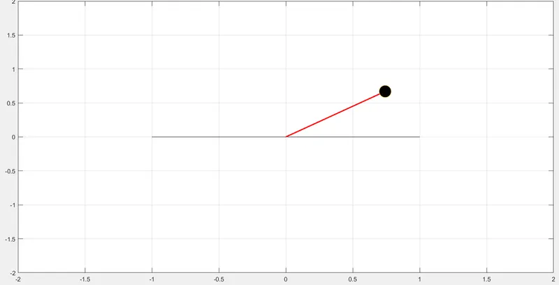
To solve this issue I have used the term (3*pi/2+) to bring the pendulum position down.

  x1= l*cos(3*pi/2+theta);
    y1=l*sin(3*pi/2+theta);

After applying the term (3*pi/2+) into x1 and y1 values, I did not face any issues regarding to the pendulum position.

SECOND ERROR:

videofile=VideoWriter('Simple_pendulum_video.avi','Uncompressed. AVI');

The mistake I had committed is a dot between uncompressed and AVI, so the animation video file was not saved due the error between the term uncompressed and AVI.

PICTURE OF THE ERROR:

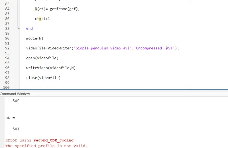
After removing the dot between the term uncompressed and AVI, I did not encounter any other issues.

I had mentioned the final result as a video link of a simple pendulum animation which will redirect to youtube.

https://youtu.be/gSfsX0XZYXE