Project 2 - Rankine cycle Simulator
AIM :
- To Create a Rankine Cycle Simulator using MATLAB.
- Code should calculate the state points of the Rankine Cycle based on user inputs.
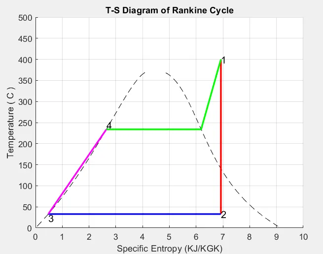
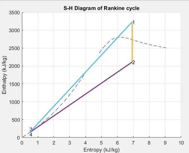
- Plot the corresponding T-s and h-s plots for the given set of inputs.
INTRODUCTION :
The Rankine cycle is an idealized thermodynamic cycle which is used to predict the performance of the Steam Turbine systems. It was also used to study the performance of the reciprocating engines such as steam locomotives.
The Rankine cycle is an idealized thermodynamic cycle of a constant pressure heat engine that converts part of heat into mechanical work. In this cycle the heat is supplied externally to a closed loop, which usually uses water as the working fluid.
The Rankine cycle power is depends on the temperature difference between the heat source (Boiler) and a cold source (Condenser).
The Source for heating in these power plants are nuclear fission or fossil fuels such as coal, Natural gas, and oil or solar power. If the temperature is high, The performance of the rankine cycle could be better.
While many substances could be used as the working fluid in the Rankine cycle but water is usually the fluid of choice due to its favorable properties, such as its non-toxic and unreactive chemistry, abundance, and low cost, as well as its thermodynamic properties. For example, water has the highest specific heat of any common substance – 4.19 kJ/kg K.
Moreover, It has very high heat of vaporization, which makes it an effective coolant and medium in thermal power plants. Changing the phase of the water is much easier than any other reactive substance and availability of a water is everwhere comparing to anyother working fluid. By considering these as crucial parameters, so Water has considered as working fluid in a Steam Turbine System.
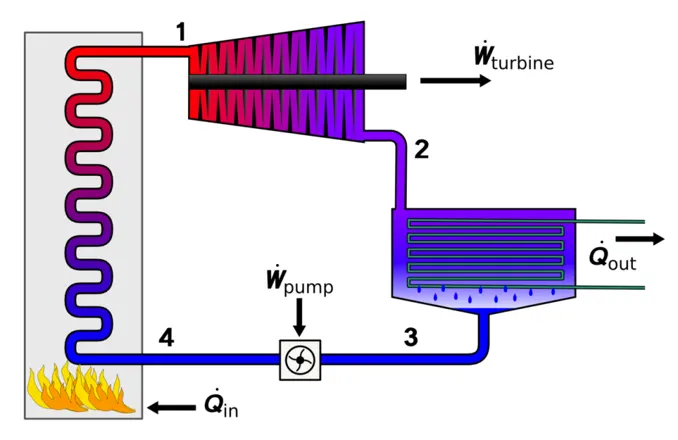
THE PROCESSES OF THE RANKINE CYCLE :
Isentropic compression :(Centrifugal pumps)
The liquid condensate is compressed adiabatically from state 1 to state 2 by centrifugal pumps (usually by condensate pumps and then by feedwater pumps). The liquid condensate is pumped from the condenser into the higher pressure boiler. In this process, the surroundings do work on the fluid, increasing its enthalpy and compressing it (increasing its pressure). On the other hand the entropy remains unchanged.
Isobaric heat addition :(Boiler)
In this phase (between state 2 and state 3) there is a constant-pressure heat transfer to the liquid condensate from an external source, since the chamber is open to flow in and out. The feedwater is heated from to the boiling point of that fluid and then evaporated in the boiler.
Isentropic expansion :( Steam turbine)
Steam from the boiler expands adiabatically from state 3 to state 4 in a steam turbine to produce work and then is discharged to the condenser (partially condensed). The steam does work on the surroundings blades of the turbine and loses an amount of enthalpy equal to the work that leaves the system.
Isobaric heat rejection :(Condenser)
In this phase the cycle completes by a constant-pressure process in which heat is rejected from the partially condensed steam. There is heat transfer from the vapor to cooling water flowing in a cooling circuit. The vapor condenses and the temperature of the cooling water increases.
MATLAB CODING FOR RANKINE CYCLE :
clear all
close all
clc

%Displaying the process statements

fprintf('\n            RANKINE CYCLE SIMULATOR \n')
fprintf('\n 1-2 is Isentropic Expansion in the Turbine\n')
fprintf('\n 2-3 is Constant pressure Heat Rejection by the condenser\n')
fprintf('\n 3-4 is Isentropic compression in the pump\n')
fprintf('\n 4-1 is Constant pressure Heat Addition by the Boiler\n')

%Formulating a code to find the rankine cycle efficiency

%Given data

% Inlet pressure of turbine

p1=input('\n Enter the pressure at the turbine inlet (In bar)=');

% Outlet pressure of turbine and inlet pressure of conderser

p2=input('\n Enter the pressure at the condenser (In bar) = ');

% Inlet temp of turbine

 t1=input('\n Enter the temperature at the Turbine inlet (In celsius) = ');


 %Calulating the state point 1

 %Find the saturated temp for given pressure

Tsat= XSteam('Tsat_p',p1);

h_c1=XSteam('h_pt',p1,t1);

h_c2=num2str(h_c1);

h_c3=h_c2(1:4);

h1=str2num(h_c3);

 s1=XSteam('s_pt',p1,t1);

 %Calculating the state point 2
 %p2=0.05

 s2=s1;

 vf=XSteam('vL_p',p2);
 vg=XSteam('vV_p',p2);
 hf=XSteam('hL_p',p2);

 %Extracting hg
 hg1=XSteam('hV_p',p2);
 h_g2=num2str(hg1);
h_g3=h_g2(1:4);

hg=str2num(h_g3);


%Extracting hfg
hfg_1=hg-hf;
 h_fg2=num2str(hfg_1);
h_fg3=h_fg2(1:4);

hfg=str2num(h_fg3);
sg=XSteam('sV_p',p2);
sf=XSteam('sL_p',p2);
sfg=sg-sf;

%s2=sf+x.sfg via of this formula the x value could be find.

% x = dryness fraction

x=((s2-sf)/sfg);

% If the value of x is less than 1 then it is a wet steam.

h2_c=hf+x*hfg;

 h2_c1=num2str(h2_c);

h2_c2=h2_c1(1:5);

h2=str2num(h2_c2);

t2= XSteam('Tsat_p',p2);


%Calculating the state point 3

h3=hf;
v3=vf;
p3=p2;
t3=t2;
s3=XSteam('sL_p',p3);

%Calculating the state point 4
%dh=Tds+Vdp

s4=s3;
%dh=h4-h3
%h4-h3=v3(p4-p3)
p4=p1;
t4=t3;
t5=XSteam('Tsat_p',p4);
s5=XSteam('sL_p',p4);
t6=t5;
s6=XSteam('sV_p',p4);

h4=v3*((p4*100)-(p3*100))+h3;

%Displaying the all the output on command window

fprintf('\n                   RESULTS       \n')
%For state point 1
fprintf('\n At state Points - 1 ')
fprintf('\n P1 = %2.2f Bar',p1)
fprintf('\n T1 =%4.2f C',t1)
fprintf('\n H1 =%4.2f KJ/Kg ',h1)
fprintf('\n S1 =%2.2f KJ/kg-C\n',s1)

%For state point 2
fprintf('\n At state Points - 2 ')
fprintf('\n P2 = %2.2f Bar',p2)
fprintf('\n T2 =%4.2f C',t2)
fprintf('\n H2 =%4.2f KJ/Kg ',h2)
fprintf('\n S2 =%2.2f KJ/kg-C \n',s2)

%For state point 3
fprintf('\n At state Points - 3 ')
fprintf('\n P3 = %2.2f Bar',p3)
fprintf('\n T3 =%4.2f C',t3)
fprintf('\n H3 =%4.2f KJ/Kg ',h3)
fprintf('\n S3 =%2.2f KJ/kg-C \n',s3)

%For state point 4
fprintf('\n At state Points - 4 ')
fprintf('\n P4 = %2.2f Bar',p4)
fprintf('\n T4 =%4.2f C',t4)
fprintf('\n H4 =%4.2f KJ/Kg ',h4)
fprintf('\n S4 =%2.2f KJ/kg-C \n',s4)


heat_added=h1-h4;
fprintf('\n Heat input is : %4.2f KJ/Kg\n', heat_added)

Turbine_work=h1-h2;
fprintf('\n Work produced by the turbine : %4.2f KJ/kg\n',Turbine_work)

heat_rejected=h2-h3;

pump_work=h4-h3;
fprintf('\n Work required by the pump :%2.2f KJ/Kg\n',pump_work)

%Find the efficiency of the rankine cycle

Wnet=(Turbine_work-pump_work);
fprintf('\n Net work done is : %4.2f KJ/Kg \n',Wnet)

eff=(Wnet/heat_added)*100;
fprintf('\n Thermal efficiency of the rankine cycle is %2.2f \n',eff)

%Back work ratio

bwr=(pump_work/Turbine_work);
fprintf('\n Back work ratio is : %2.4f\n',bwr)


%Specific steam consumption

ssc= 3600/Wnet;
fprintf('\n Specific Steam Consumption is : %2.2f Kg/Kwh\n',ssc)

%Work ratio

Work_ratio=(Wnet/Turbine_work);


%Plotting

%T-S plot
T=linspace(0,374,100);  %The value 374 is critical point of a water
figure(1);
hold on
for i = 1:length(T)
    s_l(i)=XSteam('sL_T',T(i));
    s_g(i)=XSteam('sV_T',T(i));
    h_l(i)=XSteam('hL_T',T(i));
    h_g(i)=XSteam('hV_T',T(i));

end

plot(s_l,T,'linestyle','--','color','black');
plot(s_g,T,'linestyle','--','color','black');

plot([s1 s2],[t1 t2],'linewidth',2,'color','r');
text(s1,t1,'1','fontsize',12);

plot([s2 s3],[t2 t3],'linewidth',2,'color','b');
text(s2,t2,'2','fontsize',12);

plot([s3 s4],[t3 t4],'linewidth',2,'color','y');
text(s3,t3-10,'3','fontsize',12);

plot([s4 s5],[t4 t5],'linewidth',2,'color','m');
text(s5,t5+10,'4','fontsize',12);
plot([s5 s6],[t5 t6],'linewidth',2,'color','g');

plot([s6 s1],[t6 t1],'linewidth',2,'color','g');

ylabel('Temperature ( C )')
xlabel('Specific Entropy (KJ/KGK)')
axis([0 10 0 500]);
title('T-S Diagram of Rankine Cycle')
grid on

%Plotting h-s diagram of the Rankine cycle

figure(2)


hold on

plot(s_l,h_l,'linestyle','--','color','black');
plot(s_g,h_g,'linestyle','--','color','black');
plot([s1 s2],[h1 h2],'linewidth',2)
text(s1,h1,'1');
plot([s2 s3],[h2 h3],'linewidth',2)
text(s2,h2,'2');
plot([s3 s4],[h3 h4],'linewidth',2)
text(s3,h3+100,'3');
plot([s4 s1],[h4 h1],'linewidth',2)
text(s4,h4-50,'4');
xlabel('Entropy (kJ/kg)')
ylabel('Enthalpy (kJ/kg)')
title('S-H Diagram of Rankine cycle')
grid on
EXPLAINATION OF THE CODING :
The Matlab coding starts with three important commands which are clear all, close all, clc. The objective of these commands is to clear the previous data in command window , work space and editor window.
fprintf command has used to print a particular statements in command window. In our case, we had printed the four processes of the rankine cycle.
The values of the p1, p2 and t1 need to provide in command window once the code runs. The input command will display the statement in command window which had mentioned inside the input command bracket. According to the allocated values for the input p1,p2 and t1 the rankine cycle simulation runs.
XSteam is file which has data regarding to the steam table with help of XSteam file we could extract the needed data by calling it .
Syntax for Xsteam: XSteam('Tsat_p',p1) - filename('Needed parameter', Value which matches to the needed parameter or Helping value)
By using the XSteam file the essential data can be extracted such as TSat, H , S, vf, vg , hf, hfg, hg, sg, sf , sfg, p and t.
In order to find the h2 value the x value is needed. X is a dryness fraction which helps to find either h2 is a wet steam or dry steam.
If the x is less than 1 ,then it is wet steam. If the x is 1, then it is dry steam. If the value of x is above 1, then it super saturated steam.
Once the x value is derived we could find the h2.
The s1 value is equal to the s2 value (s1 = s2).
In state point 3, the value of hf is the value of h3 and v3 is equal to the value of vf which had pulled out from the XSteam file.
The Inlet pressure of the pump and outlet of pressure of the turbine and the condenser were same (p3=p2).
The Inlet temperature of the pump and outlet temperatue of the condenser were same (t3=t2).
The s3 value can be extracted from Xsteam file.
In state point 4, the s4 value is equal to s3 value and p1 is the value for p4.
The Inlet temperature of the boiler and the outlet of the pump temperature were same (t4=t3);
The h4 value can be calculated with help of adiabatic equation.
To display all the derived parameters in command window with its respective names using fprintf command.
syntax for fprintf, fprintf(' The content which needs', Value for the content).
Via of the fprintf command the four state point values had discovered.
By Subtracting h1 with h4 will provide the heat_added value (h1-h4).
The Turbine_work value can be derived by subtracting h1 with h2 value (h1-h2).
By Subtracting h2 with h3 will provide the heat_rejected value (h2-h3).
The pump work can be caluculated by subtracting the h4 with h3 value.
By dividing the Wnet value with heat_added value will determine the efficiency of the rankine cycle. Multiplying the obtained efficiency value with 100 will show the efficiency of the rankine cycle in percentage.
To calculate the back work ratio the pump_work should divide by the turbine work value.
The Specific steam consumption parameter can be calculated by dividing 3600/ Wnet value.
Plotting the T and S data values for the four state points will display the graphical view of the T and S data.
Here, Linspace command has used to split and find the values for temperature(T) from 0 - 374.
For loop is command used to describe the saturation curve for the plot.
Plotting the s_l and s_g with temperature(T) will display the saturation temperature curve in the plot.
Linestyle command is used to determine the appearance of the line in the plot.
Color command will determine the color of the line.
Plotting the s1 and s2 with t1 and t2 will display graphical view of data for s and t.
Repeating the same process for the four state points s and t will display the graphical over view of the S - T plot.
Hold on command will bring multiple plots which is regarding to the single figure.
The H-S plotting process is very similar to S-T plot format. By replacing the T value with H value and adding some parameters will bring the H-S plots.
Text command is used to describe the name of the line.
xlabel is used to name the x-axis.
ylabel is used to name the y-axis.
Title command is used to name the plot.
Grid on command is used to highlight the line for each value in x and y axis for easy understanding.
PICTURE OF OUTPUT IN COMMAND WINDOW :
Entering the crucial parameters to run the simulation:
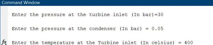
According the feeded data for the parameters of p1, p2, t1, the rankine cycle simulation runs.
RESULTS OF THE RANKINE CYCLE :
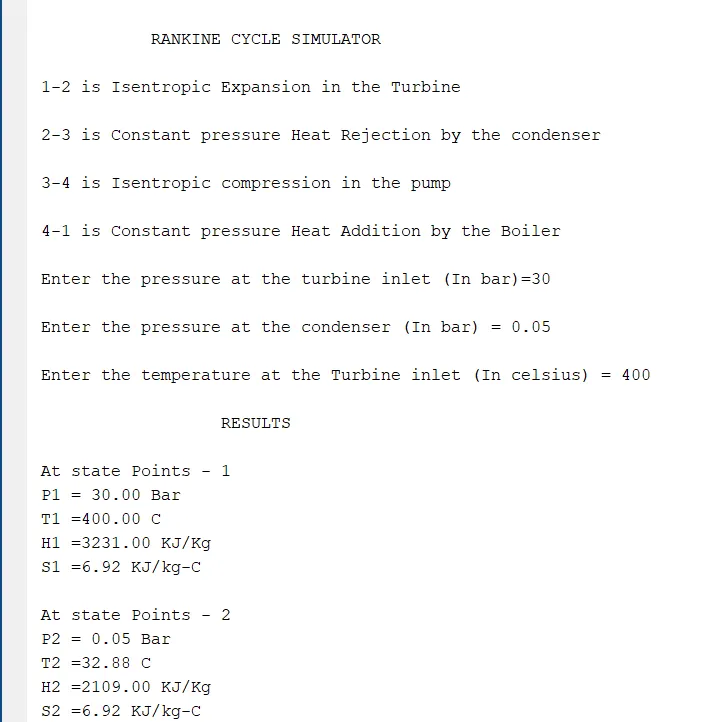
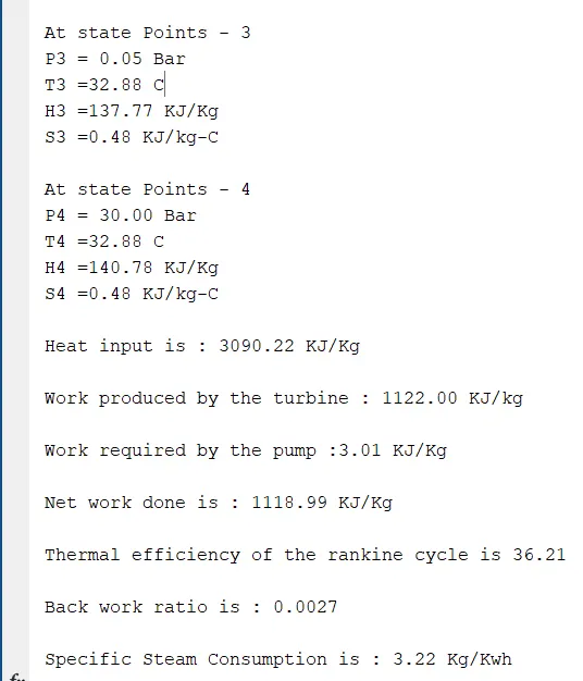
OUTPUT OF THE PLOTS :
APPLICATION OF THE PROJECT :
The project automates the method of manually problem solving process into an automated solving process and work as simulation for rankine cycle. By following this project format, Any problem can be automated and get an output in a numerical form and graphical view according to the applied data. This automated process has achieved with aid the of MATLAB software.
CONCLUSION :
By Modifying the certain codes depends on the problem will simulate the respective problem and provide the both numerical and graphical view for easy understanting about the data.