Week 3 - Solving second order ODEs
Aim: To write a program that solves the ODE represents the equation of motion of a simple pendulum with damping
Objectives:
To animate the motion of the pendulum with the position of the pendulum as a function of time.
Given:
The ode equation
In the above equation,
use,
L=1 metre, length of the pendulum
m=.1 kg, mass of the ball
b=0.05 damping coefficient.
g=9.81 m/s2. gravity
condition given
Time=20 sec,
Initial value at time =0 are:
Initial angular displacement=0,
Initial angular velocity=3 rad/sec
CODE:
clear all
close all
clc
%given input parameter
b=.05;  %damping coefficient
g=9.81; %gravity in m/s2
l=1;    %length of the pendulum in m
m=.1;    %mass of the ball in kg

%initail condition
theta_0=[0;3]; %initial despacement as zero and initial velocity as 3 rad/s

%time points
t_span= linspace(0,20,200); % time array ranging from 0 to 20 second with 200 points

%solve ODE
[t, results]= ode45(@(t,theta) ode_func(t, theta, b,g,l,m),t_span,theta_0);% time,position = ode45(@function, time,

figure(1)
plot(t,results(:,1))
hold on
plot(t,results(:,2))
xlabel('time')
ylabel('displacement & velocity')
legend('displacement','velocity')
x0=0;
y0=0;
ct=1;
figure(2)

for i= 1:length(results(:,1))
    ang1= results(i);

     x1= -(l*sin(ang1));
     y1= -(l*cos(ang1));


%plotting

plot(x1,y1,'o','markersize',20,'markerfacecolor','m')
line([x0 x1],[y0 y1],'linewidth',1,'color','k')
line([-0.5 0.5],[0 0],'linewidth',5,'color','[0.8500 0.3250 0.0980]')
axis([-1 1  -2 1])
pause(0.03)
M(ct)=getframe(gcf);
ct=ct+1
end

movie(M)
videofile=VideoWriter('pendulum_simulation.avi','UnCompressed AVI');
open(videofile)
writeVideo(videofile,M)
close(videofile)
Function:
function [dtheta_dt] = ode_func_damper(t,theta,b,g,l,m)
 theta1 = theta(1)
 theta2 = theta (2)
 dtheta1_dt = theta2;
 dtheta2_dt =-(b/m)*theta2-(g/1)*sin(theta1);
 dtheta_dt = [dtheta1_dt; dtheta2_dt];
end
Step-wise explanation of code:-
Clearing screen and workspace
- It is always important to start with clear all, close all and clc command in MATLAB M-scrip since
- clc:cleans up the command window and now one can work without getting confused with the commands for previous runs
- Clear:erases the variables from previous runs this will reduce chances of error in subsequent runs and the programmer does not have to worry about unnecessary trash variables.
- Close all:closes all currently open figures. This can be very helpful during subsequent runs of the same script. If the figure from the previous run has not been closed then the subsequent run will plot the data on the already open figure. Which of course is a total waste.
Defining the inputs and values:-
- The given input value are assigned to respective variables ‘b’ as damping coefficient, ‘g’ as gravity, ‘l’ as length, ‘m’ as mass of the ball.
- The initial condition angular displacement and angular velocity are defined as a column matrix in the variable theta_0 and the values are 0 and 3 rad/sec.
- t-span is the variable used in ode solver which specify the iterations that to solve ode.
- The t-span is define in array with linspace command where 0 to 20 sec.
Defining the ODE solver:-
- The ode45 is a function in MATLAB that solves Ordinary Differential Equation using numerical methods. In this problem we have the highest order of 2, so we take simplify the equation into simple differential equation by converting to two constant values.
- The syntax for the ode45 function is
[t,y] = ode45(@(t,y) 2*t, t_span, y0);
- Here the y is replaced with result variable, 2*t is replaced with ode_function of the damper which is explained below, and y0 e is replaced with theta_0.
Explaining ode_func( t, theta, b, g, l, m)
- This function simplifies the seconder order differential equation to first order by creating two ODEs, 1st ode is dtheta1_dt and 2ns one is dtheta2_dt. By transforming the second order to first order it is easy to differentiate the equation.
- Then the ode45 function solves this simple differential equation.
Plotting velocity and displacement in graph:
- Figure command creates figure graphics objects. figure objects are the individual windows on the screen in which MATLAB displays graphical output. figure creates a new figure object using default property values. since we are want two output plots for pendulum oscillation, velocity and displacement plotting.
- The figure(1) command is used to display the velocity and displacement plot with reference to time.
- The plot is made using plot command, the displacement is plotted with first column of result matrix and velocity is plotted with second column.
Plotting pendulum oscillation:
- The figure(2) command is used to display the pendulum oscillation position with reference to time.
- Ct is a variable used for counting, for loop is used to animated the position of the pendulum for each position
- Since one end of the pendulum string is fixed initial point x0 and y0 are set to the origin.
- The other end position is located with the formula shown below.
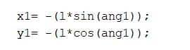
- The marker command is used to draw a ball on the plot with respect to the points.
- Line command is used to draw the string.
Animating the pendulum motion and store as video file:
- Movie command is used to create an animated movie of plots. The video writer command is used to create a video file in the working folder followed open, writevideo and close command to write the video with plot frames.
Errors faced while programming:
I encounter error with plot with not displaying the line i.e. the string is not displayed in the plot after running the program.
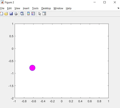
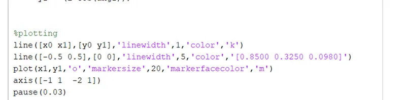
Then I understood the need why plot command is executed before line command. Since plot is a graphical command it displays only the graphical image with deleting other graphical image on the screen where else the line command is line object which may add the line to the current axes without deleting other graphics objects.

Then I replaced the line commands after plot commands.
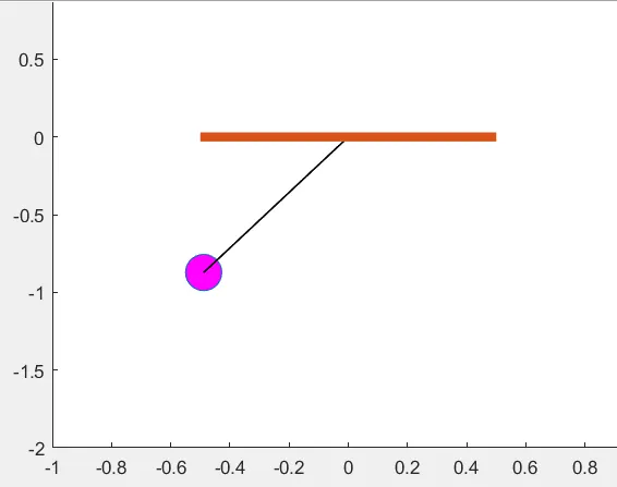
OUTPUT:
the below graph shows the displacement(blue color line) and velocity(red color line) with respect to time
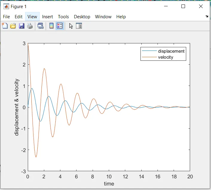
in the graph the displacement of the pendulum starts at zero and velocity start at 3 rad/sec.
the pendulum oscillation is animated and link is given below.
link:
https://drive.google.com/file/d/1zxFESJYqdyrc32Nz5jY5hub1TtG9BYh9/view?usp=sharing