Week 3 - Solving second order ODEs

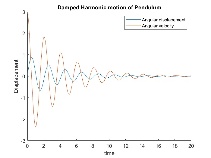
PENDULUM ANIMATION:-

Click here to watch the animation of damped harmonic motion of pendulum

STEP WISE EXPLANATION OF CODE

clearvars - clear all the previous variables of workspace

close all - close all the previous plots

clc - clear the command window

In input values of damping coefficient,acceleration due to gravity,length of pendulum,mass of bob are provided

for the simulation of pendulum between 0-20 sec. at t=0 sec.(initial condition),theta=0 and angular velocity=3 rad/sec. also provided

For solving ODE, ode45 inbuild MATLAB function has used

Next with the help of plot command the plot between time and displacement has been draw.

Next for loop has used to animate the to and fro motion of pendulum,Maker command has used to give size and color to the bob.With the help of plot command we have created horizontal support and string of the pendulum.

To make movie of this animation,movie command has used.

VideoWriter command has used to assign video format to the videofile which is in .avi

open command has used to open the video,writevideo command has used to write the video with plot frames.

finally close command has used to close the video

% programm to solve 2nd order ode

clearvars
close all
clc

% inputs
b=0.5;  % damping coefficient
g=9.81; % kg/m^2
l=1;    % in m
m=1;    % in kg
% initial condition

% angular displacement is 0 and angular velocity is 3 rsd/s
theta_0=[0;3];

% time span
t_span=linspace(0,20,400);

% solving ODE
[t,results]=ode45(@(t,theta) ode_func(t,theta,b,g,l,m),t_span,theta_0);

% plotting
figure(1)
hold on 
plot(t,results(:,1))
plot(t,results(:,2))
title('Damped Harmonic motion of Pendulum')
legend('Angular displacement','Angular velocity')
xlabel('time')
ylabel('Displacement')

ct=1;
for i=1:length(results(:,1))
    x_start=0;
    y_start=0;
    x_end=l*sin(results(i,1));
    y_end=-l*cos(results(i,1));
 
    % plotting the annimation of pendulum
    figure(2)
    
    plot([-1 1],[0 0],'linewidth',5)
    hold on
    plot([x_start x_end],[y_start y_end],'linewidth',3)
    hold on
    plot(x_end,y_end,'o','MarkerSize',20,'MarkerFaceColor','b')
    title('Animation of transient behaviour of pendulum')
    axis([-1.5 1.5 -1.5 1])
    pause(0.03)
    hold off

    M(ct)=getframe(gcf);
    ct=ct+1;
end
movie(M)
videofile=VideoWriter('Pendulum Animation.avi','Uncompressed AVI');
open(videofile)
writeVideo(videofile,M)
close(videofile)

​

function [dtheta_dt]=ode_func(t,theta,b,g,l,m)

theta1=theta(1);
theta2=theta(2);
dtheta1_dt=theta2;
dtheta2_dt=-(b/m)*theta2-(g/l)*sin(theta1);
dtheta_dt=[dtheta1_dt;dtheta2_dt];

end