Week 3 - Solving second order ODEs

import math
import matplotlib.pyplot as plt
import numpy as np
from scipy.integrate import odeint
def ODE(theta,t,b,g,l,m):
    theta1 = theta[0]
    theta2 = theta[1]
    dtheta1_dt = theta2
    dtheta2_dt = -(b/m)*theta2-(g/l)*math.sin(theta1)
    dtheta_dt = [dtheta1_dt,dtheta2_dt]
    return dtheta_dt
b = float(input('Enter damping constant: '))
g = 9.81
l = float(input('Enter length of the pendulum (in m): '))
m = float(input('Enter the mass of the pendulum bob (in kg): '))
a = int(input("Initial time point:"))
c = int(input("Final time point:"))
n = int(input("No. of Intervals:"))
e = int(input("Enter the initial point: "))
f = int(input("Enter the final point: "))
theta_0 = [e,f]
t = np.linspace(a,c,n)
theta = odeint(ODE,theta_0,t,args=(b,g,l,m))
plt.figure(1)
plt.plot(t,theta[:,0],'b-',label=r'$Displacement$')
plt.xlabel('Time')
plt.ylabel('Plot')
plt.legend(loc='best')
plt.show()
plt.figure(2)
plt.plot(t,theta[:,1],'r--',label=r'$Velocity$')
plt.xlabel('Time')
plt.ylabel('Plot')
plt.legend(loc='best')
plt.show()
plt.figure(3)
plt.plot(t,theta[:,0],'b-',label=r'$Displacement$')
plt.plot(t,theta[:,1],'r--',label=r'$Velocity$')
plt.xlabel('Time')
plt.ylabel('Plot')
plt.legend(loc='best')
plt.show()
P = theta[:,0]
B = 1
X0 = 0
Y0 = 0
for i in P:
    X1 = X0 + (l*math.sin(i))
    Y1 = Y0 - (l*math.cos(i))
    B = B+1
    filename = str(B)+'.png'
    plt.figure()
    plt.plot([-2,2],[0,0],'b-',linewidth=2)
    plt.plot([X0,X1],[Y0,Y1])
    plt.plot(X1,Y1,'o',markersize=20)
    plt.xlim([-2,2])
    plt.ylim([-2,2])
    plt.title('Simple Pendulum Motion Simulation')
    plt.savefig(filename)

CODING THE PENDULUM MOTION SIMULATION:

1. Import 'math', 'matplotlib.pyplot' as 'plt', 'numpy' as 'np' and 'odeint' from 'scipy.integrate' respectively.
2. Use 'def' command to define the function 'ODE' and declare the variables necessary to simulate the motion of the pendulum. Also give the expressions and conditions required to calculate the values for the variables.
3. Give the inputs required to simulate the motion of the pendulum by solving the 2nd order ODE using the commands, 'input', 'int' and 'float'.
4. Use the 'odeint' command to solve the 2nd order ODE and obtain the data to plot the displacement and velocity graphs.
5. By using 'plt.plot' command and the values obtained from the previous step, plot the displacement vs time graph.
6. Repeat the same process to obtain the nelocity vs time graph.
7. Combine the steps 5 and 6 to obtain the comparative graph of diaplacement and velocity vs time.
8. Initiate a counter, 'B' and give the initial x and y coordinates as 0.
9. Give the required conditions and expressions to translate the next x and y coordinates.
10. Give an increment to the counter such that after each execution of the 'for' loop, the next frame is obtained.
11. Plot the obtained data by giving the 'xlim' and 'ylim' as [-2,2] and give the tile as 'Simple Pendulum Motion'. Save the obtained figures by using 'plt.savefig'.

RESULTS

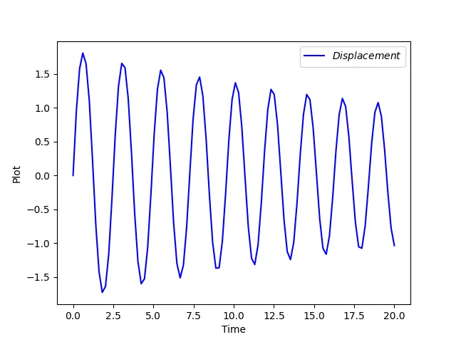
Displacement vs. Time graph

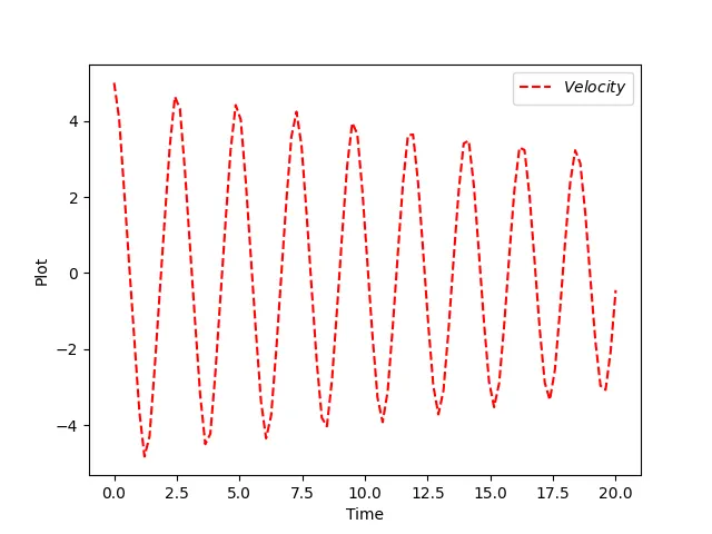
Velocity vs. Time graph

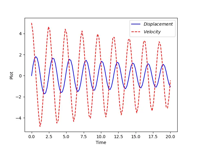
Comparative graph of Displacement and Velocity vs. Time

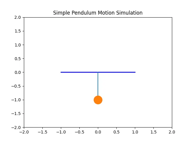
Simulation of the motion of the simple pendulum