Week 3 - Solving second order ODEs

SOLVING SECOND ORDER ODE's

AIM: To write a program to solve an ordinary differential equation(ODE) and to animate the motion of the pendulum using MATLAB.

OBJECTIVE:
*To write a program to solve the ODE using ode solver function
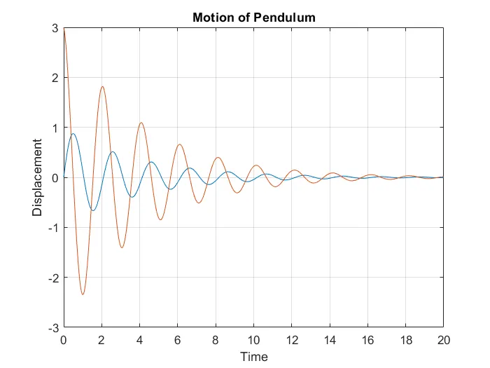
*To plot the graph of angular displacement vs time and angular velocity vs time
*To animate the motion of the pendulum.

THEORY:
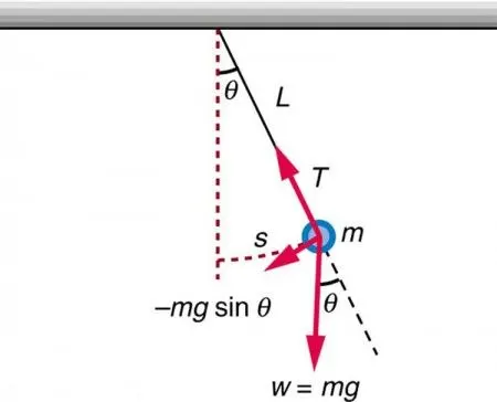
A simple pendulum consists of a mass m hanging from a string of length L and fixed at a pivot point P. When displaced to an initial angle and released, the pendulum will swing back and forth with periodic motion.

An ordinary differential equation(ODE) contains the derivative of an unknown function. The ordinary differential equation is an equation having variables and a derivative of the dependent variable with reference to the independent variable.

The second order ordinary differential equation(ODE) of a simple pendulum is given by ,

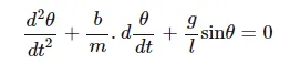
where , b= damping coefficient
m=mass of the bob,kg
g=acceleration due to gravity,m/s^2
l=length of the string,m

By breaking down the above second order differential equation,we get

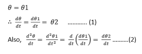
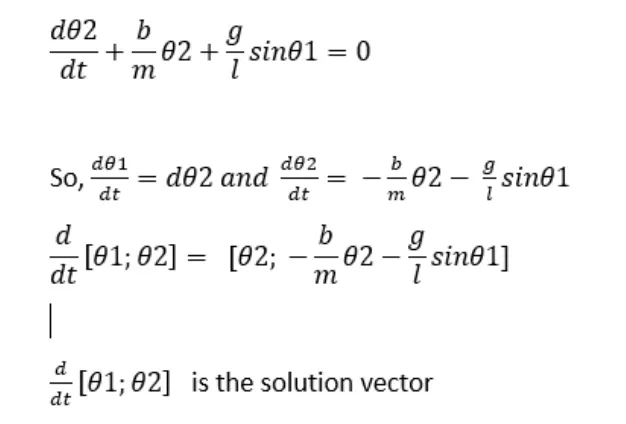
by substituting (1) and (2) in the equation we get,

INPUTS:
b=0.05
m=1 kg
g=9.81 m/s^2
L=1 meter

CONDITIONS:
Angular velocity=3 rad/sec
Angular displacement=0
Time motion:0-20 sec

PROGRAM:

close all
clc

b=0.05;
g=9.81;
l=1;
m=0.1;

%initial conditions
theta_0=[0;3];

%time_span
t_span=linspace(0,20,500);

%solve ode
[t,results]=ode45(@(t,theta) ode_func(t,theta,b,g,l,m), t_span, theta_0);

plot(t,results(:,1))
hold on
plot(t,results(:,2))
xlabel('Time')
ylabel('Displacement')
title('Motion of Pendulum')
grid on


%creating a for loop to make the animation
theta=results(:,1);
ct=1;
for i=1:length(results(:,1))
    Theta1=theta(i);
    %initial coordinates
    x0=0;
    y0=0;

    %final coordinates
    x1=l*sin(Theta1);
    y1=-l*cos(Theta1);

    %Plotting the base of the pendulum
    plot([-1,1],[0,0],'LineWidth',6,'color','m')
    hold on 
    %plotting the string 
    plot([x0,x1],[y0,y1],'LineWidth',4,'color','g')
    hold on
    %plotting the bob of the pendulum
    plot(x1,y1,'o','MarkerSize',20,'MarkerFaceColor','b')
    hold off
    axis([-3 3 -2 2])
    grid on 
    pause(0.03)
    M(ct)=getframe(gcf);
    ct=ct+1;
end

%Conversion of animation into movie
movie(M);
videofile=VideoWriter('pendulum.avi','uncompressed avi');
open(videofile);
writeVideo(videofile,M)
close(videofile)

%ODE function
function [dtheta_dt] = ode_func(t,theta,b,g,l,m)


theta1=theta(1);
theta2=theta(2);
dtheta1_dt=theta2;
dtheta2_dt=-(b/m)*theta2 - (g/l)*sin(theta1);
dtheta_dt=[dtheta1_dt;dtheta2_dt];

end

PROCEDURE:
*Firstly, the "close all", "clc" commands were used."close all" command is used to close all the current figures and "clc" command is used to clear all the inputs and outputs from the command window.
*The next step is to define the inputs of the simple pendulum such as damping coefficient(b),acceleration due to gravity(g),length of the string(l),and mass of the bob(m).
*The next step is to define the initial conditions of the simple pendulum such as angular displacement,angular velocity,time motion.
*'t_span' command was used.It is a command used in ODE45 solver which specifies the time span of the iterations.Here the time taken is 0-20 seconds and has 500 values between them.
*The next step is to solve the ODE by using ODE45 function. ODE45 is usually the function of choice among the ODE solvers.This function compares methods of orders four and five to estimate error and determine step size.The results are stored in an array of row matrix of two columns.
*The [t,results] is the function handle of the anonymous function.It means that the results have been determined with respect to time.
*The anonymous function we used here is ode_func(t,theta,b,g,l,m).Using the ODE45 command,the function is solved.
*To create a specified set of points to keep the bob at different locations, the 'for' loop is used.
*Initial coordinates were defined (x0,y0) which are the coordinates for the fixed point at one end of the string.Final coordinates(x1,y1) were also defined.They denote the different positions of the bob.
*"ct" command was used to count each and every position and stores the data.
*A 'pause' command was used to pause the command for a certain time.Here we have used 0.03 seconds.
*The movie command(M) was used to capture each and every frame for everytime the 'for' loop runs.
*The next step of the loop is to add +1 to the 'ct' command.
*'End' command was used to end the for loop from running.
*To create an animation of the pendulum, the Movie command(M) was used.
*'videoWriter' command was used to assign the videoformat.Here,'avi' format was used.
*'open' command is used to open the video file.
*'Writevideo'command was used to write the video with plot frames.
*'close' command was used to close the videofile.

GRAPH:

ANIMATION VIDEO:

https://drive.google.com/drive/folders/1NtELJB1f63dBWml9qY4eCqjCXgRCzKat?usp=sharing

ERROR FACED DURING EXECUTION OF CODE:

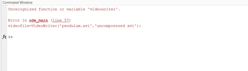
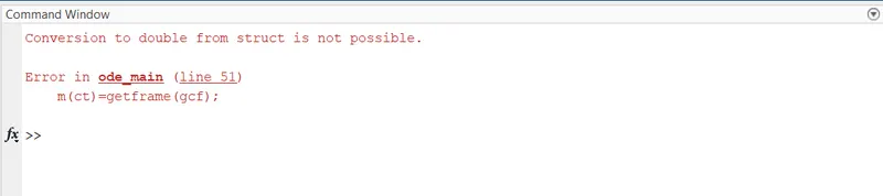
The error I faced while doing this program was usage of uppercase letters in 'Movie' command and failed to execute the function due to case sensitivity in 'VideoWriter' function.

STEPS TAKEN TO OVERCOME THOSE ERRORS:
*I checked the syntax and performed the execution of code again.
*I watched the video to make sure there is no mistake.
*I checked the functions I used here are case-sensitive.

RESULTS:
*The angular dispacement vs time and angular velocity vs time graphs were plotted.
*The animation video for the motion of the pendulum was created using the software "MATLAB".