Week 3 - Solving second order ODEs
Solving Second Order ODE-Simple Pendulum (MATLAB)
Aim :
To write a program to solve the second order ODE of motion of a simple pendulum with damping.
Objective :
1) Solve the second order ODE of a simple pendulum into first order ODE.
2) write a program that simulate the simple pendulum motion.
3) Create the Animation video file of pendulum motion and save the animation video file in hard disk.
Theory :
Behaviour of a Simple Pendulum :
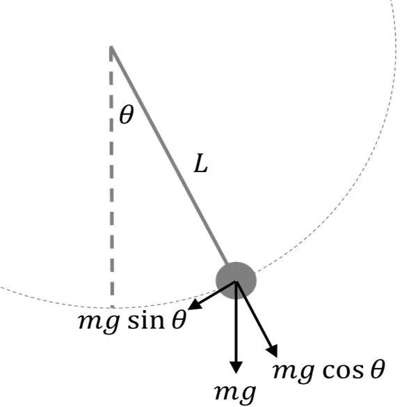
A pendulum is a body suspended from a fixed support which swings freely back and forth under the influence of dravity. When a pendulum is displaced from its initial position, It is subjected to a restoring force due to gravity which will accelerate the pendulum back to its initial or equilibrium position. When released the restoring force in the pendulum's mass causes it to oscillate about the equilibrium position swinging back and forth.
A simple pendulum refers to an ideal model where the "bob" of mass 'm' is suspended by a massless/weightless cord or an string.
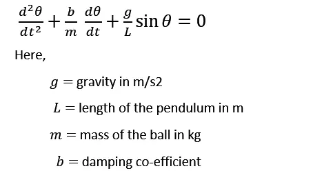
The Second Order ODE equation for a pendulum is given as.
This Second Order ODE equation can be breaked into several First order ODE
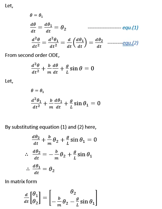
This matrix form is the solution vector of this simple pendulum. here, "theta 1" and "theta 2" are contains the input vector.
Given Input data :
- Length of the pendulum (L) = 1 m
- Mass of the ball (m) = 1 kg
- damping co-efficient (b) = 0.05
- gravity (g) =9.81 m/s2
Initial codition :
motion time (t) is 0 to 20 sec
Angular Velocity = 3 rad/s
Angular Displacement = 0
Function Program :
In order to find out pendulum movement we need to solve Solution vector as input data of theta 1 and theta 2 in matlab by using Function program.
This function code as follows,
function [dtheta_dt] = ode_fun(t,theta,b,m,l,g)
theta1=theta(1);
theta2=theta(2);
dtheta1_dt=theta2;
dtheta2_dt=-(b/m)*theta2-(g/l)*sin(theta1);
dtheta_dt=[dtheta1_dt;dtheta2_dt];
end
Syntax ODE 45 :

Description :
[t,y] = ode45(ode fun,tspan,y0)
Where, tspan = [t0 tf], integrates the system of differential equation y'=f(t,y) from t0 to tf with the initial conditions y0. Each row in the solution array y corresponds to a value retruned in column vector t. All MATLAB ODE solver can solvers can solve system of equations and proble that involve a mass matrix.
ode45 is a versatile ODE solver and is the first solver you should try for most problems.If the proble is requires high accuracy, then there are other ODE solvers that might be better suited to the problem.
Program - ODE Program :
Now write a program for find the motion of simple pendulum by using ode45 code in MATLAB.
%program for solve higher order ODE
clear all
close all
clc

%inputs
b=0.05;
m=1;
l=1;
g=9.81;

%initial condition
theta_0=[0;3];

%time periode
t_span=linspace(0,20,700);

%solving ODE
[t,result]=ode45(@(t,theta)ode_fun(t,theta,b,m,l,g),t_span,theta_0);

%plotting graph time vs Displacement and Angular velocity

figure(1)
hold on
plot(t,result(:,1),'color',[0.5 0.5 0],'linewidth',1)   % color code [Red green Blue]
plot(t,result(:,2),'color','b','linewidth',1)
hold off
xlabel('Time-Sec')
ylabel('Angular velocity and Displacement')
legend('Displacement','Angular velocity')

%plotting graph Displacement vs Angular velocity

figure(2)
plot(result(:,1),result(:,2))
xlabel('Displacement')
ylabel('Angular velocity')

%to create an animation

theta3=result(:,1);
ct=1;
for i=1:length(theta3);
     THETA3=theta3(i);
     l=1;
     x0=0;
     y0=0;
     x1=l*sin(THETA3);
     y1=-(l*cos(THETA3));

figure(3)
plot([-1 1],[0 0],'color','b','linewidth',3);          %Pendulum Support
hold on
plot([0 0],[0 0],'o','color','m','markersize',7);      %Pendulum Hinge
hold on
plot([x0 x1],[y0 y1],'color','r','linewidth',2);       %Pendulum String
hold on
plot(x1,y1,'o','markerfacecolor','m','markersize',20); %Pendulum Bob
hold off
grid on
axis([-1.5 1.5 -1.5 0.5 ])
pause(0.002)
M(ct)=getframe(gcf);
ct=ct+1;
end
%creating movie
movie(M)
videofile=VideoWriter('pendulum_animation.AVI','uncompressed AVI');
open(videofile)
writeVideo(videofile,M)
close(videofile)
Code Explanation :
1) The first step is to clear all old data and graphs using "clear all", "close all" and "clc" commands.
2) Next take the given inputs and the initial condition as the input to the program for theta_0=[0;3] are the initial codition of displacement and velocity of pendulum. And time array given by linspace command.
3) Then write the Function Program for solve the solution vector seperately. As we discussed above matlab inbuilt function (ode45) used to solve and find out the motion of simple pendulum with the given initial condition.
4) In next step result of solved ODE is plotted with respect to time using plot command.
5) The first figure 1 is to plot graph for "Time vs Displacement and Angular Velocity" by using plot, hold on, xlable ,ylable and legend commands.
6) The figure 2 is to plot graph for "Displacement vs Angular Velocity" by using plot, hold on, xlable ,ylable and legend commands.
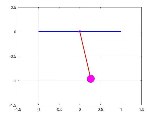
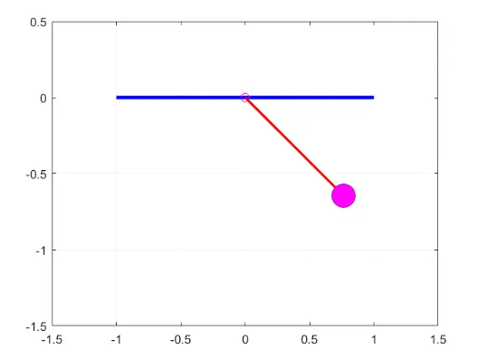
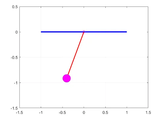
7) The next step is to create an Animation video of a simulate the pendulum motion. Create the loop for find out the each movement of pendulum by using "for" loop.
8) Next is to plot pendulum support by using plot, color, linewidth commands. For Pendulum Hinge by using plot, color, markersize commands. For Pendulum String by using plot, color, linewidth commands. For pendulum Bob by using plot, color, markersize commands are used.
9) In the next step is to create the Animated video of the oscillating pendulum by using the "movie(M)" and save the video file in hard disk.
10) Animation Video :
1) A new set of values is defined as theta3 which contains the set of values of result array of column1 for position values. ct stands for counder in this program it refers to the 1st iteratin of inputs ct=1.And ct=ct=1 at the end stands for next set of iterations so it icremating counter untill the last to simulate.
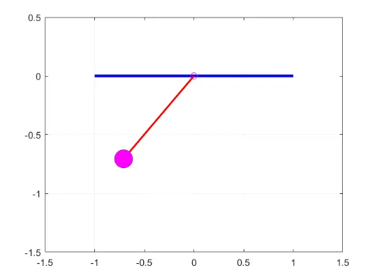
2) The for loop is to support the iterations untill the last to simulate. 4 different plot commands are used to plot support, hinge,string and bob respectively. these plot cammands are controled by hold on, hold off commands to avoid overwritting of plots.
3) The pause command is used to have a interval between frames (0.002s). And for create movie use movie(M) command. next set the video file name and format of the video by using the command VideoWriter('pendulum_animation.AVI', 'uncompressed AVI')
4) next step is to open video file and write video by the command writevideo(videofile,M) and close video file by using the command close.
Outputs :
Figure 1 : Plot graph Time vs Displacement and Angular Velocity.
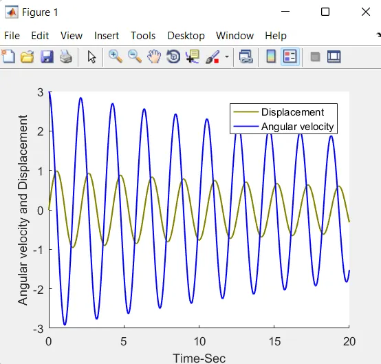
Figure 2 : Plot graph Displacement vs Angular Velocity.
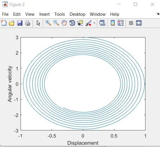
Figure 3 : Animation video of oscillating pendulum and screenshot of it.
Animation Video link :
Conclusion :
In this way with the use of MATLAB study of motion of simple pendulum with damping can be studied with the help of plots and animation video , Similarly we can solve other higher differential equations and its solution can be obtained easily.