Week 3 - Solving second order ODEs
ODE is used to describe the transient behavior of a system. simple pendulum is an example of ode.
The way the pendulum moves depends on the Newtons second law. When this law is written down, we get a second order Ordinary Differential Equation that describes the position of the "ball" with respect to time. there are multiple ode systems. here we are to see the second order ode system.
we are to make a second order ode system for simple pendulum and animate the final result.
MAIN CODE:
#we are to take in the important modules for the function to understand the commands
#the modules are
#math helps in basic math operations
import math
# matplotlib helps in plotting of the results
import matplotlib.pyplot as plt
#numpy helps in the arrays proper addition
import numpy as np
#scipy helps in the better ode, integration operations etc...
from scipy.integrate import odeint

def sode(theta,time,b,l,g,m):
	theta1 = theta[0]
	theta2 = theta[1]
	dtheta1_dt = theta2
	dtheta2_dt = -(b/m)*theta2 - (g/l)*math.sin(theta1)
	dtheta_dt = [dtheta1_dt,dtheta2_dt]

	return dtheta_dt

#inputs to the function
#the gravity as we all know (m/s^2)
g = 9.81
#damping value for the pendulum
b = 0.05;
#mass of the object (kg)
m = 1
#length of the pendulum(m)
l = 1

#the displacement and the veloicty at the start are
first_inputs = [0,3]
time = np.linspace(0,20,300)

#ode function main process
theta = odeint(sode,first_inputs,time,args = (b,l,g,m))

plt.plot(time,theta[:,0],'r-',label='displacement')
plt.plot(time,theta[:,1],'b--',label='velocity')
plt.legend()
plt.xlabel('time')
plt.ylabel('displacement vs velocity')
plt.show()


ct = 1
#the attached end of pendulum
x0 = 0
y0 = 0
for i in theta[:,0]:
	#the free end of pendulum
	x1 = l*math.sin(i)
	y1 = -l*math.cos(i)

	file = 'ode%05d.png'%ct
	ct = ct+1
	plt.figure()
	plt.plot([-1.5,1.5],[0,0],'r',linewidth=6)
	plt.plot([x0,x1],[y0,y1],'b',linewidth=3)
	plt.plot(x1,y1,'o',markersize=25)
	plt.xlim([-2,2])
	plt.ylim([-2,1])
	plt.savefig(file)
EXPLANATION OF THE MAIN CODE:
we are taking in the important modules for the system to understand the commands we give in.
the important modules for the ode system are math, matplotlib, numpy, scipy. these form the very basic requirement of the ode system.
#we are to take in the important modules for the function to understand the commands
#the modules are
#math helps in basic math operations
import math
# matplotlib helps in plotting of the results
import matplotlib.pyplot as plt
#numpy helps in the arrays proper addition
import numpy as np
#scipy helps in the better ode, integration operations etc...
from scipy.integrate import odeint
this here is the function code for the ode system to understand it core idea.
the def contains the name,the intakes like theta angles, time for which the operation has to happen, b, l, g, m.
def sode(theta,time,b,l,g,m):
theta 1 is stated with 1st value of theta and theta 2 is given the 2nd value of theta. since we are using python the index point starts from 0 and so the the value of1 stays in index 0.
theta1 = theta[0]
theta2 = theta[1]
the major formula is breaken down for better understanding
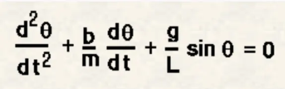
this second order ode is made into two lower order odes
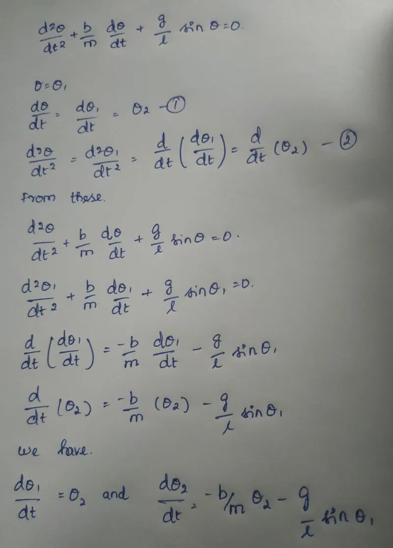
which is then written as
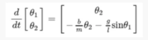
this formula is written as input
dtheta1_dt = theta2
dtheta2_dt = -(b/m)*theta2 - (g/l)*math.sin(theta1)
dtheta_dt = [dtheta1_dt,dtheta2_dt]
the value of dtheta_dt is made as output.
return dtheta_dt
the physical inputs like the gravitational force on the pendulum, damping acting on it, mass of the pendulum, and the length are stated below.
#inputs to the function
#the gravity as we all know (m/s^2)
g = 9.81
#damping value for the pendulum
b = 0.05;
#mass of the object (kg)
m = 1
#length of the pendulum(m)
l = 1
this is the values of the initial displacement and the velocity of the pendulum.
0 is for displacement and 3 for velocity.
#the displacement and the veloicty at the start are
first_inputs = [0,3]
time for which the modeling is processing is given below.
from 0 to 20 with 300 divisions in between them.
time = np.linspace(0,20,300)
the first major ode code is used here to take the output theta value.
#ode function main process
theta = odeint(sode,first_inputs,time,args = (b,l,g,m))
the plotting is done for the displacement and the velocity of the pendulum. the plot differentiation command like legend, xlabel and y label are made to display.
plt.plot(time,theta[:,0],'r-',label='displacement')
plt.plot(time,theta[:,1],'b--',label='velocity')
plt.legend()
plt.xlabel('time')
plt.ylabel('displacement vs velocity')
the plot is made visible with the help of plt.show().
plt.show()
the ct helps in achieving the saving of different figures of the process.
ct = 1
the attached end of the pendulum is stated as below
#the attached end of pendulum
x0 = 0
y0 = 0
for the animation of the pendulum the for loop command is used
the free oscillating ends as stated as x1 a nd y1.
for i in theta[:,0]:
#the free end of pendulum
x1 = l*math.sin(i)
y1 = -l*math.cos(i)
this helps in storing the individual images with their own respective names for better id.
file = 'ode%05d.png'%ct
the ct helps in as above stated by incrementing the values and storing different datas.
ct = ct+1
plotting is done for animation.
plt.figure()
the fixed and free ends are plotted.
plt.plot([-1.5,1.5],[0,0],'r',linewidth=6)
plt.plot([x0,x1],[y0,y1],'b',linewidth=3)
marker is used in showing the bottom weight of the pendulum.the axis limits are stated and the files are made to store in their names.
plt.plot(x1,y1,'o',markersize=25)
plt.xlim([-2,2])
plt.ylim([-2,1])
plt.savefig(file)
PLOT FOR THE CODE:
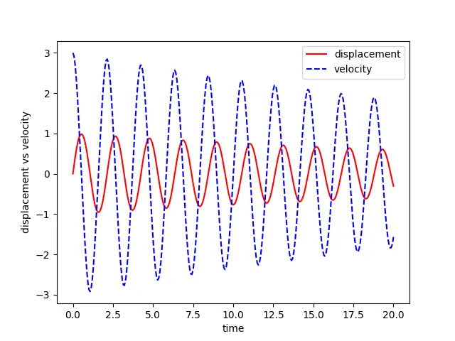
THIS SHOWS AS THE TIME INCREASE THE VELOCITY AND DISPLACEMENT SLOWS DOWN.
THE IMAGES OF THE SIMPLE PENDULUM STORED UNDER THEIR NAMES FOR ANIMATION:
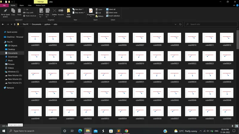
THESE IMAGES ARE STITCHED TO FORM AN ANIMATION OF THE MOVING PENDULUM.
ERRORS:
1.indentation mistakes.
2.linspace was stated without stating numpy at front.
3.the y value is stated as +l and so the animation was inverted
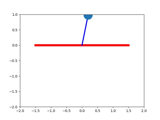
these issues are later corrected for the right output.
CONCLUSION:
the plotting is done and the animation of the pendulum is done.
ANIMATION:
YOUTUBE:https://youtu.be/tG40ntck0WU