Week 3 - Solving second order ODEs

WEEK 3: SOLVING SECOND ORDER ODE

AIM: Write a program in Matlab\Octave that will simulate the pendulum motion and also solve the second order ODE that represents the motion of pendulum.

THEORY:

A pendulum is a body suspended from a fixed support so that it is free to swing back and forth under the influence of gravity. When a pendulum moves laterally from its rest and equilibrium positions, it undergoes a restoring force due to gravity, which accelerates towards the equilibrium position. When released, the restoring force on the pendulum's mass causes it to oscillate about the equilibrium position, rotating it back and forth. The math of pendulums is generally quite complicated. in the case of a simple pendulum, the equations of motion can be solved analytically for small-angle oscillations.

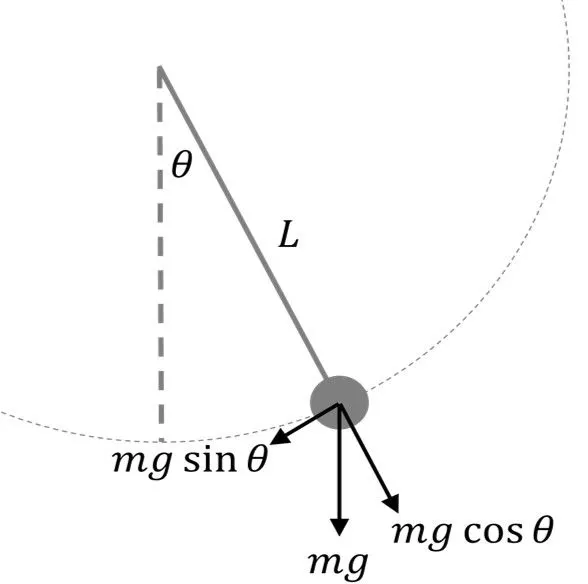
A simple gravity pendulum is an idealized mathematical model of a real pendulum.This is a weight on the end of a massless cord suspended from a pivot, without friction. Since in this model there is no frictional energy loss, when given an initial displacement it will swing back and forth at a constant amplitude. The model is based on these assumptions:

• The rod or cord on which the bob swings is massless, inextensible and always remains taut.
• The bob is a point mass.
• Motion occurs only in two dimensions, i.e. the bob does not trace an ellipse but an arc.
• The motion does not lose energy to friction or air resistance.
• The gravitational field is uniform.
• The support does not move.

The differential equation which represents the motion of a simple pendulum is

`(d^2theta)/ dt^2+{g/l }sin theta =0`

where g is the magnitude of the gravitational field, ℓ is the length of the rod or cord, and θ is the angle from the vertical to the pendulum.

PROCEDURE:

1. We used ode45 function to solve the second order ODE of the simple pendulum.
2. But first a function is created to reduce the second order ODE to first order equations.
3. After reducing the second order ODE to first order form, we use the following commands in our main code to use the ode45 function: [t,y] = ode45(odefun,tspan,y0)

The code shown below is used as function.

function [dtheta_dt] = ode_f(t,theta,b,g,l,m)
  theta1 = theta(1)
  theta2 = theta(2)
  dtheta1_dt = theta(2);
  dtheta2_dt = -(b/m)*theta2-(g/l)*sin(theta1);
  dtheta_dt = [dtheta1_dt; dtheta2_dt];
end

The main codes is as follows:

clear all
close all
clc

%SECOND ORDER ODE FOR MOTION OF SIMPLE PENDULUM

%REQUIRED DATA IN SI UNITS
b = 0.05;  %damping coefficient
l = 1;     %lenght of the pendulum
m = 1;     % mass of the bob
g = 9.81;  % gravity

%inital condition
theta_0 = [0;3]; %angular displacement and angular veolcity at t=0

%Time span
t_span = linspace(0,20,500);

%Using ode45 solver and also using function
[t , results] = ode45(@(t,theta) ode_f(t,theta,b,g,l,m),t_span,theta_0);

%Plotting Angular Displacement and Angular Velocity w.r.t Time
figure(1)
hold on
plot(t,results(:,1))
plot(t,results(:,2))
title('Simple harmonic motion of pendulum')
xlabel('Time(sec)')
ylabel('Displacement and velocity')
legend('Angular Displacement','Angular Velocity')
grid on 
hold off

%Animating the motion of pendulum
ct =1;
for i=1:length(t_span)
    x0=0;
    y0=0;
    
    x1= l*sin(results(i,1));
    y1= -l*cos(results(i,1));
    
    figure(2)
    plot([-1 1], [0 0],'linewidth',3)
    hold on
    plot([x0 x1],[y0 y1],'linewidth',1.5)
    hold on
    
    plot(x1,y1,'marker','o','markersize',15,'markerFacecolor','y')
    title('Motion of Pendulum')
    axis([-1.5 1.5 -1.5 1])
    pause(0.03)
    hold off
    
    M(ct)= getframe(gcf)
    ct= ct+1;
    
end
movie(M)
videofile=VideoWriter('pendulum.mp4','MPEG-4');
open(videofile)
writeVideo(videofile,M)
close(videofile)    


    

OUTPUT:

• We get the desired output graph of angular displacement and velocity.
  
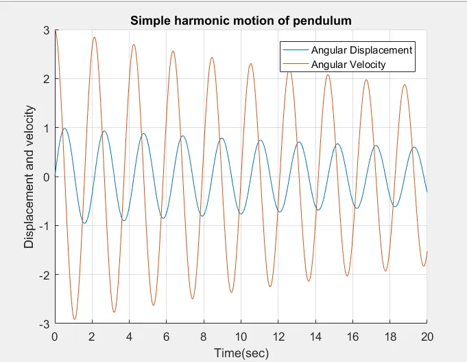
• The required animation file is attached below along with the code.

CONCLUSION:

• Use of ode45 function was successfully implemented as we got the desired output.
• Learnt the use of ode45 function in matlab.