Week 3 - Solving second order ODEs

Aim:

To solve the program of second order ODE of the given equation using MATLAB Software, to animate the oscillation of pendulum by the results of ODE equation solved.

Procedure:

The given ODE represents the equation of motion of a simple pendulum with damping in which,

Inputs given as below

L=1m length of the pendulum in m,

m=1kg mass of the ball in kg,

b=0.05 damping coefficient.

g=9.81 gravity in m/s2

t = motion of pendulum between 0 to 20,

Angular Displacement=0,

Angular Velocity=3 rad/sec at time t=0

Coding:

By using the above inputs need to do program for second order ODE as below.

%Pendulum oscillation
clear all
close all
clc

% input variables
b=0.05;
g=9.81;
l=1;
m=1;
l1=3;

% initial conditions
theta_0= [0;3];


% time points
t_span = linspace(0,20,700);

% solve ode
[t, s] = ode45(@(t,theta) ode_func(t, theta, b, g, l, m), t_span, theta_0);

x = [l1*sin(s(:,1))];
y = [-l1*cos(s(:,1))];



tiledlayout(2,1)
nexttile
hold on
plot(t,s,'LineWidth',2);
xlabel('Time');
ylabel('Plot');
legend('angular displacement','angular velocity');
hold off

nexttile
h3 = plot([0,x(1,1)],[0,y(1,1)],'color','blue',Marker='.',MarkerSize=20,LineWidth=2);
hold on
h4 = plot(x(1),y(1),'.','color','red','markersize',40);
line = plot([-1 1],[0 0],'color','cyan','LineWidth',3)
xlabel('X-Axis');
ylabel('Y-Axis');
axis([-8 3 -8 3]);
% ht = title('Time: '+t(1)+' sec');
hold off

ct=1
for id = 1:length(t)
    set(h3(1),XData=[0,x(id,1)],YData=[0,y(id,1)])
    set(h4,XData=x(id),YData=y(id))
%     set(ht,String='Time: '+t(id)+' sec')
    pause(0.03);
    M(ct) = getframe(gcf);
    ct=ct+1

end
    

movie(M)
videofile = VideoWriter('Pendulum oscillation.avi', 'Uncompressed AVI')
open(videofile)
writeVideo(videofile,M)
close(videofile)

In the above coding,

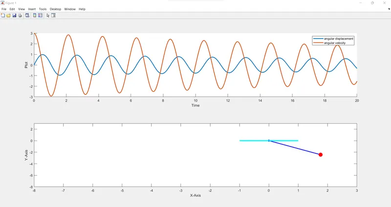
The command 'tiledlayout(2,1) represents the two output graphs on the same window, as tile(1) represents the graph of angular displacement and angular velocity and tile(2) represents the oscillation movement of the pendulum which is used as an 'nexttile' command before plotting the graphs.

The command 'marker' represents the size of the marker or size of the pendulum.

The command 'legend' used to highlight the line difference in graph 1.

ode_func Coding as below,

function [dtheta_dt] = ode_func(t, theta, b, g, l, m)
theta1 = theta(1);
theta2 = theta(2);
dtheta1_dt = theta2;
dtheta2_dt = -(b/m)*theta2 -(g/l)*sin(theta1);
[dtheta_dt] = [dtheta1_dt; dtheta2_dt]
end

After the Coding, click 'Run' icon to simulate the coding in order to get the result file.

Output:

On behalf of the entered coding we will get the results as below.

The animated video file has been uploaded in youtube, link is attached as below.

Youtube Link: https://youtu.be/MlArOp0wN-k

First Graph Result:

The Orange line represents the angular velocity with respect to time as initially the velocity given is 3rad/s

The blue line represents the angular displacement with respect to time as initially the displacement of pendulum is 0.

As X-axis represents the Time.

Y-axis represents the Velocity.

Second Graph Result:

The Cyan line represents the Fixing area or the damping area of the pendulum,

The Pendulum oscillates with respect to time and displacement solved in ODE equation.

Result:

The above coding and output result file shows to solve the program of second order ODE of the given equation using MATLAB Software and also to animate the oscillation of pendulum by the results of ODE equation solved.