Project 2 - Rankine cycle Simulator

Aim:

To create a Rankine Cycle Simulator using MATLAB, understanding Rankine theory, reading files form XSteam data.

Procedure:

To Simulate a Rankine cycle using MATLAB, to understand the concept of Rankine cycle.

Rankine Cycle:

In Thermodynamics, Rankine cycle was first developed in 1859 by Scottish Engineer William.J.M Rankine, this cycle is used within the boiler, converting water into steam in which expands through the turbine producing useful work, this cycle converts the heat into mechanical energy in which this useful energy is converted into the electrical energy.In this process an idealized cycle is simulated, hence neglecting losses that occurs in during heat transfer.This cycle is manly driven out from Carnot Cycle where its power will depends on the temperature difference between the heat source & a cold source, the more the difference in temperature the more the mechanical heat can be extracted. Efficiency of Rankine cycle is limited by high heat of vaporization of working fluid, friction losses. Water is usually the fluid of choice due to its non-toxic and unreactive chemistry, abundance and low cost of its thermodynamic properties. By condensing the working steam vapour to a liquid the pressure at the turbine outlet is lowered and the energy required by the feed pump consumes less than 3% of turbine output power & these factor contribute to a higher efficiency for the cycle. The benefits of this is offset by the low temperature of steam admitted to the turbine.

Process and Stages of Rankine Cycle:

• Isentropic Expansion in the Turbine.
• Constant Pressure Heat Rejection in Condenser
• Isentropic Compression in the Pump
• Constant Pressure Heat Addiction in the Boiler.

Working of Rankine Cycle Simulator:

Stage 1-2:

The dry saturated vapour expands through a turbine , generating the power. This decreases the temperature and pressure of the vapour and some condensation will occur.

Stage 2-3:

The vapour-liquid mixture leaving the turbine(2) is condensed at low pressure, usually in a surface condenser using cooling water. In well designed and maintained condenser the pressure of the vapour is wee below the atmospheric pressure, approaching the saturation pressure of the operating fluid at the cooling water temperature.

Stage 3-4:

The pressure of the condensate is raised in the feed pump. Because of the low specific volume of liquids, the pump work is relatively small and often neglected in thermodynamic calculations.

Stage 4-1:

High Pressure liquid enters the boiler from the feed pump(4) and is heated to the saturation temperature (on the saturation curve). Further addicted of energy cause evaporation of the liquid until it is fully converted to saturated steam(1) or superheated(1).

As the water condenses in the condenser, waste heat is given off in the form of water vapour which can be seen billowing from a plant’s cooling towers. This waste heat is necessary in any thermodynamic cycle. Due to this condensation step, the pressure at the turbine outlet is lowered. This means the pup requires less work to compress the water-resulting in higher overall efficiencies.

Coding as below:

% Rankine Cycle Simulator
% Objective to simulate the rankine cycle
% Plot t-s, h-s graph using Xsteam data
% Water & steam properties according to IAPWS IF-97
clear all
close all
clc

disp('RANKINE CYCLE SIMULATOR');
disp('1-2 Isentropic Expansion in the turbine');
disp('2-3 Constant Pressure Heat rejection in the condenser');
disp('3-4 Isentropic compression in the pump');
disp('4-1 Constant pressure heat addition in the boiler');

% Obtaining input data as follows
p1 = input('enter the preesure at the turbine inlet(in bar)p1:');
p2 = input('enter the preesure at the condensor(in bar)p2:');

t1 = input('enter the temperature at the turbine inlet(in degree celsius)t1:');

fprintf('rRESULTSrn')

% stage1 turbine inlet
s1 = XSteam('s_pT',p1,t1);
h1 = XSteam('h_pT',p1,t1);

% stage2 condensor inlet
sf2 = XSteam('sL_p',p2);
sg2 = XSteam('sV_p',p2);
hf2 = XSteam('hL_p',p2);
hg2 = XSteam('hV_p',p2);

s2 = s1;
t2 = XSteam('Tsat_p',p2);

% splitting the formula

x2 = ((s2-sf2)/(sg2-sf2));
h2 = hf2+(x2*(hg2-hf2));

% stage3 pump inlet
p3 = p2;
t3 = XSteam('Tsat_p',p2);
s3 = XSteam('sL_p',p3);
h3 = XSteam('hL_p',p3);

cp4 = XSteam('cpL_p',p3);
cv4 = XSteam('cvL_p',p3);
gamma = (cp4/cv4);
g = (gamma-1)/gamma;

% stage4 boiler inlet

p4 = p1;
s4 = s3;
h4 = XSteam('h_ps',p4,s4);
t4 = t3*((p4/p3)^g);

% turbine work

wt = h1-h2

% pump work

wp = h4-h3;

% network

w_net = wt-wp;

% heat in and out of system

q_in = h1-h4;
q_out = h2-h3;

n = w_net/q_in;
np = n*100;

SSC = 3600/w_net;
tf_sat = XSteam('Tsat_p',p1);
sf_sat = XSteam('sL_p',p1);
hf_sat = XSteam('hL_p',p1);
sg_sat = XSteam('sV_p',p1);
hg_sat = XSteam('hV_p',p1);

% plot figure 1
figure(1)
hold on
temp = linspace(0,400,1000);
for i = 1:length(temp)
    aa(i) = XSteam('sL_T',temp(i));
end

for j = 1:length(temp)
    bb(j) = XSteam('sV_T',temp(j));
end

plot(aa,temp,'color','g')
plot(bb,temp,'color','g')

temp = (XSteam('Tsat_p',p1));
t0 = linspace(temp,t1,300);
for i = 1:length(t0)
    c11(i) = XSteam('s_pt',p1,t0(i));
end

t5 = XSteam('Tsat_p',p4);
s5 = XSteam('sL_T',t5);

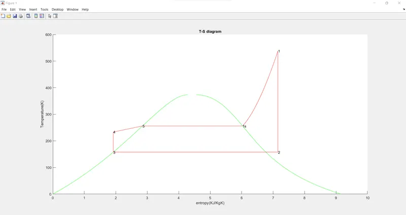
plot([s1 s2],[t1 t2],'color','r')
plot([s2 s3],[t2 t3],'color','r')
plot([s3 s4],[t3 t4],'color','r')
plot([s4 s5],[t4 t5],'color','r')
plot([sf_sat sg_sat],[tf_sat tf_sat],'color','r')
plot(c11,t0,'color','r')

title('T-S diagram')
xlabel('entropy(KJ/KgK)')
ylabel('Temperature(K)')

text(s1,t1,'1');
text(s2,t2,'2');
text(s3,t3,'3');
text(s4,t4,'4');
text(s5,t5,'5');
text(sg_sat,tf_sat,'1s');

% plot figure 2
figure(2)
hold on
temp1 = linspace(0,400,1000);
for i = 1:length(temp1)
    cc(i) = XSteam('hL_T',temp1(i));
end

for j = 1:length(temp1)
    dd(j) = XSteam('hV_T',temp1(j));
end

plot(aa,cc,'color','g')
plot(bb,dd,'color','g')

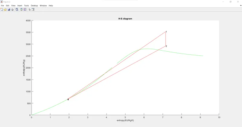
plot([s1 s2],[h1 h2],'color','r')
plot([s2 s3],[h2 h3],'color','r')
plot([s3 s4],[h3 h4],'color','r')
plot([s4 s1],[h4 h1],'color','r')

title('H-S diagram')
xlabel('entropy(KJ/KgK)')
ylabel('enthalpy(KJ/Kg)')

text(s1,h1,'1');
text(s2,h2,'2');
text(s3,h3,'3');
text(s4,h4,'4');

% printing output

% State Point 1
disp('RESULTS')
disp('at stage point 1:');
fprintf('P1 is : %f barn',p1);
fprintf('T1 is : %f deg celsium',p1);
fprintf('T1 is : %f KJ/Kgn',h1);
fprintf('S1 is : %f KJ/KgKrn',s1);

% State Point 2
disp('at state point 2:');
fprintf('P2 is : %f Barn',p2);
fprintf('T2 is : %f deg celsiusn',t2);
fprintf('H2 is : %f KJ/Kgn',h2);
fprintf('S2 is : %f KJ/KgKrn',s2);
fprintf('X is : %f rn',x2);

% State Point 3
disp('at state point 3:');
fprintf('P3 is : %f Barn',p3);
fprintf('T3 is : %f deg celsiusn',t3);
fprintf('H3 is : %f KJ/Kgn',h3);
fprintf('S3 is : %f KJ/KgKrn',s3);

% State Point 4
disp('at state point 4:');
fprintf('P4 is : %f Barn',p4);
fprintf('T4 is : %f deg celsiusn',t4);
fprintf('H4 is : %f KJ/Kgn',h4);
fprintf('S4 is : %f KJ/KgKrn',s4);

fprintf('Wt : %f KJ/Kgn',wt);
fprintf('Wp : %f KJ/Kgn',wp);
fprintf('Wnet : %f KJ/Kgn',w_net);
fprintf('SSC : %f KJ/KWhbn',SSC);

Output:

T-S Diagram:

H-S Diagram:

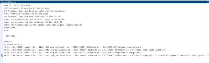
Command Window:

Conclusion:

From the above coding and procedure it is clear to perform a Rankine Cycle Simulator with given data, output of T-S curve & H-S curve is obtained and attached.