Week 3 - Solving second order ODEs

%A program that solves the following ODE of Simple Pendulum.

`(d^2 θ)/(dt^2 )+b/m dθ/dt+g/L sin⁡θ=0`

%Programs

%Function Program

function [dtheta_dt] = ode_func(t,theta,b,g,l,m)

theta1 = theta(1)
theta2 = theta(2)
dtheta1_dt = theta2;
dtheta2_dt = -(b/m)*theta2-(g/l)*sin(theta1);
dtheta_dt = [dtheta1_dt;dtheta2_dt];
end

%Main Program

clear all
close all
clc

b = 0.05;%Damping coefficient
g = 9.81;%Gravity(m/s^2)
l = 1;%Length of the pendulum(m)
m = 1;%Mass of the ball(kg)

%Initial condition
theta_0 = [0;3];

%Time points
t_span = linspace(0,20,1000);

%Solving ODE
[t,results] = ode45(@(t,theta) ode_func(t,theta,b,g,l,m),t_span,theta_0);

%Plotting 
figure(1)
plot(t,results(:,1))
hold on 
plot(t,results(:,2))
ylabel('Angular Velocity and Displacement')
xlabel('Time')

%Plotting Angular velocity VS Position  
figure(2)
plot(results(:,1),results(:,2))
xlabel('Position')
ylabel('Angular Velocity')
ct = 1 %Initial counter value

for i = 1:length(t_span)
% Hanging position of pendulum   
x0 = 0;
y0 = 0;

%Movement of pendulum
x1 = l*sin(results(i,1));
y1 = -l*cos(results(i,1));

figure(3)
%Plotting hanging Point
plot(x0,y0,'s',MarkerFaceColor='g',MarkerSize=10)
hold on
%Defining Axis
axis([-1 1 -1.5 0])

%PLotting pendulum line
plot([x0 x1],[y0 y1],'linewidth',4,'color','b')

%Plotting pendulum ball
plot(x1,y1,'o','MarkerFaceColor','r','MarkerSize',20)

%Labelling Axis
xlabel('Angular Displacements')
title('Pendulum Simulation')
hold off
grid on

%Frame capturing
M(ct) = getframe(gcf);
ct = ct+1;%Incrementing ct 
end

%Animation of the simulation of a pendulum oscillation
movie(M)
%Creating video file
videofile = VideoWriter('pendulum_animation.avi','Uncompressed AVI');
open(videofile)
writeVideo(videofile,M)
close(videofile)

% Explanation

% Theory

A Simple Pendulum consists of a mass m hanging from a string of length L and fixed at a pivot point P.

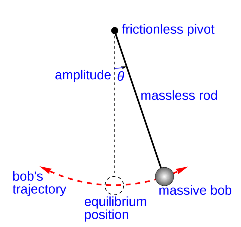
When displaced to an initial angle and released, the pendulum will swing back and forth with periodic motion. By applying Newton's second law for rotational systems, the equation of motion for the pendulum may be obtained.

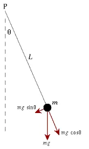
`τ=Iα`

`-mg sin⁡θ L=mL^2 (d^2 θ)/(dt^2 )`

And it will be rearranged as

`(d^2 θ)/(dt^2 )+g/L sinθ=0`

But we are going to simulate the program of Damped oscillation that’s why we are going to consider damping coefficient ().

`(d^2 θ)/(dt^2 )+b/m dθ/dt+g/L sin⁡θ=0`

b = Damping coefficient

m = Mass (`kg`)

g = Gravity (`m/s^2`)

L = Length (`m`)

`dθ/dt` = change in `θ` w.r.t. time which can also be known as velocity.

`(d^2 θ)/(dt^2 )`= change `θ` in w.r.t times square which significates the displacement.

Let us assume

`θ=θ_1`

`dθ/dt=(dθ_1)/dt=θ_2`

So,

`(d^2 θ)/(dt^2 )=(d^2 θ_1)/(dt^2 )=(d^2 θ_1)/(dt^2 )=d/dt.(dθ_1)/dt=(dθ_2)/dt`

Let’s consider the initial equation,

`(d^2 θ)/(dt^2 )+b/m dθ/dt+g/L sin⁡θ=0`

Replacing the all-derived values we get,

`(dθ_2)/dt+b/m θ_2+g/L (sin⁡θ_1)=0`

`(dθ_2)/dt=-b/m θ_2-g/L (sin⁡θ_1)`

`d/dt ((θ_1),(θ_2)) =((θ_2),(-b/m θ_2-g/L sin⁡θ_1 ))`

We have written the final equation in matrix form which is nothing but the value of, `(dθ_1)/dt` and `(dθ_2)/dt`.

% Program Explanation

Firstly, we are going to discuss the function program. Function which we have used in ode45 command.

We are going to define the function. While defining the function make sure that the name of the function and the program should be same otherwise it will not work. Also make sure to mention all the quantities that are needed so that it will be easy to understand.

function [dtheta_dt] = ode_func(t,theta,b,g,l,m)

We have to replace the changes that we have made. We are just going to replace as we done in formula.

dtheta1_dt = theta2;

dtheta2_dt = -(b/m)*theta2-(g/l)*sin(theta1);

dtheta_dt = [dtheta1_dt;dtheta2_dt];

Now we are going to discuss our Main program.

clear all- command used to clear variables from the workspace.

close all- command used to close all plot windows.

Clc-command used to clear command window.

Now we going to input some values to the program as given in the question

Damping coefficient (b) = 0.05;

Gravity (g) = 9.81`m/s^2`;

Length of pendulum rod (l) = 1m;

Mass (m) = 1kg;

As per given in the question we are going to consider angular displacement = 0 and angular velocity = 3 rad/sec. as shown below first we are going to input the angular displacement value and them we are going to input the angular velocity value in a square ([]) bracket. And we are going to put semicolon(;) in between so that it will be inputted in column form.

theta_0 = [0;3];

As per the question they have asked us to simulate the motion between 0-20 sec. that’s why we have considered the time between 0 to 20. And we are going to use linspace command here so that we can equi-space between those two intervals .

t_span = linspace(0,20,1000);

Now we are going to discuss the ODE45 function. While introducing ODE45 we have to specify that our equation is function of t and theta. Then we are going to introduce our function program that we have discussed above in which we have specified all our formulas. As our equation is a function of time and theta we will mention ‘t_span’ and ‘theta_0’ in the end. This commands output will be saved in [t,results].result contains 1000X2 means 1000 rows and 2 columns. In which first column of result consist angular displacement and second column consists of angular velocity.

[t,resuts] = ode45(@(t,theta) ode_func(t,theta,b,g,l,m),t_span,theta_0);

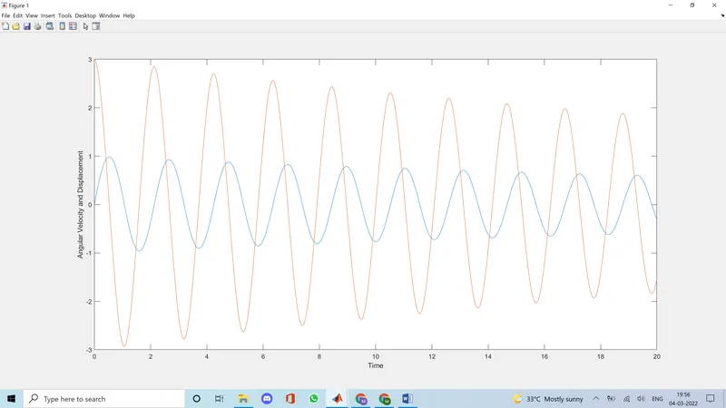
Now we are going to plot the graphs for angular displacement and angular velocity respectively. First plot command that we see will plot 1 column and all rows from the result matrix. Which means it will plot the graph for Angular displacement. And similarly, we can say that second plot command will plot the graph for Angular velocity. We are going to use hold on command in between so that we can see both plots on same graph.

plot(t,resuts(:,1))

hold on

plot(t,resuts(:,2))

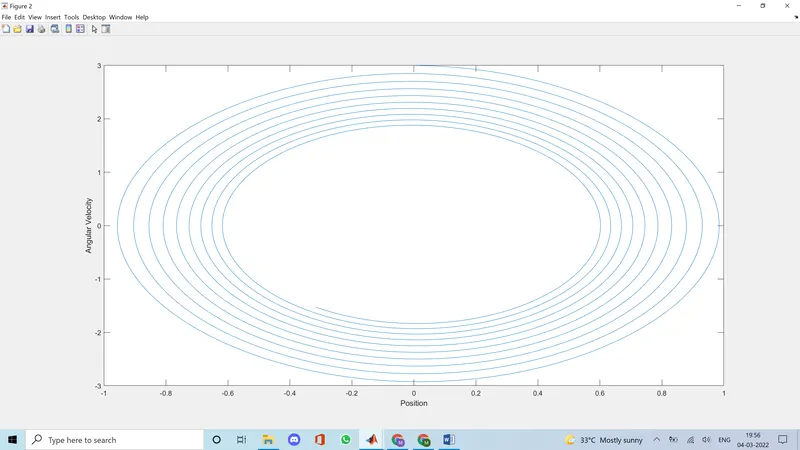
To trace the position of pendulum with respect to angular velocity we are going to use the plot command as shown below.

plot(resuts(:,1),resuts(:,2))

We are going to add one more variable to the input section of the program. Ct means counter. We are going to introduce ct variable just before the for loop so that it can be used in it further.

ct = 1

Moving further we are introducing for loop in our program. Firstly we are going to discuss the command i = 1:length(t). (:) sign denotes ‘TO’. It basically mean for i = 1 to 1000(1000 because t is a matrix which contains 1000 values).

for i = 1:length(t_span)

In next step we are going to specify the co-ordinates of hanging position of pendulum. Starting point will be origin (0,0)

x0 = 0;

y0 = 0;

we are going to specify our [x1 y1] we are going to take x and y component of only first column results. That’s why we have written results(i,1). Because we have to simulate angular displacement.

x1 = l*sin(results(i,1));

y1 = -l*cos(results(i,1));

To plot the hanging point for the pendulum we are going to use below command

plot(x0,y0,'s',MarkerFaceColor='g',MarkerSize=10)

hold on

To plot the line joining (x0,y0) and (x1,y1) we are going to use our standard command to plot the line.

plot([x0 x1],[y0 y1],'linewidth',4,'color','b')

To plot the pendulum ball we are going to use below plot command in which ‘o’ will create the sphere at given point and ‘MarkerFaceColor’ command will decide the color of sphere and similarly ‘MarkerSize’ will decide the size of marker.

plot(x1,y1,'o','MarkerFaceColor','r','MarkerSize',20)

Here we are going to know more about why we used ct in the program. So getframe returns a movie frame. The frame is a snapshot (pixmap) of the current axes or figure. To record the frames we will use the following command.

M(ct) = getframe(gcf);

As initial value of ct=1 if we add 1 to it then it will be 2. So it will record second iteration and so on.

ct = ct+1;

Movie(M) plays the movie frames in array M once

movie(M)

VideoWriter creates a videowriter object to write video data to an AVI file with motion JPEG compression. After assigning that we will open the file and write the video data as discussed above and we will close the video file.

videofile = VideoWriter('pendulum_animation.avi','Uncompressed AVI');

open(videofile)

writeVideo(videofile,M)

close(videofile)

% Plots

% Plot 1

% Plot 2

% Youtube Lin