Week 2- 2R Robotic Arm Challenge

% A program to simulate the forward kinematics of a 2R Robotic arm

% A program to plot forward kinematics of a 2R robotic arm manipulator

% Forward kinematics of a 2R robotic arm manipulator
clear all
close all
clc

% Inputs
l1 = 1;
l2 = 0.5;

theta1 = 45;
theta2 = 30;

% Coordinates
x0 = 0;
y0 = 0;

x1 = l1*cosd(theta1);
y1 = l1*sind(theta1);

x2 = x1 + l2*cosd(theta2);
y2 = y1 + l2*sind(theta2);

% Plotting
line([x0 x1],[y0 y1],'linewidth',3,'color','b')
line([x1 x2],[y1 y2],'linewidth',3,'color','g')

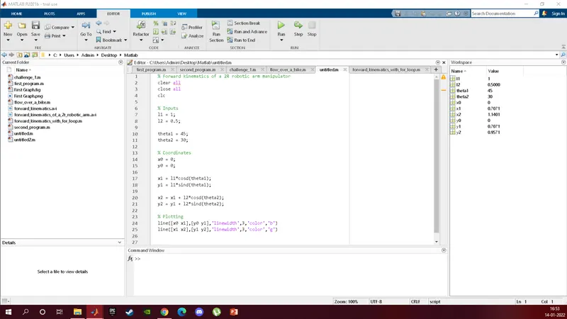
• We start the program with clear all, close all and clc. We are taking a 2 arm robot with arm 1 (l1) of 1m and arm 2 (l2) of 0.5m. The angle between the ground and l1 is theta1 and the angle between l1 and l2 is theta2.
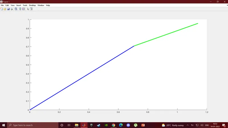
• In this program, we just plot the robot arm position for specific values of theta1 and theta2. We've taken theta1 45 degrees and theta2 30 degrees.
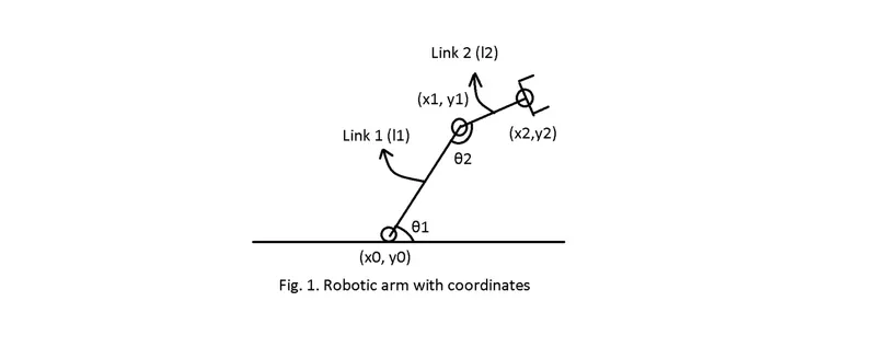
• I have drawn a robotic arm with coordinates (Fig.1) to better understand the coordinates points ((x0, yo) (x1, y1) (x2, y2)). Now with the help of Fig.1 and basic geometry, we take x0 and y0 as '0' as they start at the origin and take x1 = l1*cosd(theta1) and y1 = l1*sind(theta1) and take x2 = x1 + l2*cosd(theta2) and y2 = y1 + l2*sind(theta2). While inputting the coordinates we take 'cosd(theta)' and 'sind(theta)' because we are taking theta value in degrees.
• As there are two arms i.e two different lines we use line command instead of the plot command. Now we saved and tested the program and got the output.
• But this program can only take single values of theta1 and theta2. So to animate the output we need multiple values of theta1 and theta2. Therefore we are writing another program.

% Final program to simulate the forward kinematics of a 2R Robotic arm

clear all
close all
clc

% Inputs
l1 = 1;
l2 = 0.5;
theta1 = linspace(0,90,5);
theta2 = linspace(0,90,5);

% Loop
ct = 1;
for i = 1:length(theta1)
    THETA1 = theta1(i)
    for j = 1 : length(theta2)
        THETA2 = theta2(j)
        
        % Coordinates
        x0 = 0;
        y0 = 0;

        x1 = l1*cosd(THETA1);
        y1 = l1*sind(THETA1);

        x2 = x1 + l2*cosd(THETA2);
        y2 = y1 + l2*sind(THETA2);

        % Plotting
        plot([x0 x1],[y0 y1],[x1 x2],[y1 y2],'linewidth',3)
        axis([0 1.5 0 1.5])       
        pause(0.01)
        M(ct) = getframe(gcf);
        ct = ct+1;

    end
end

% Creating_videofile
movie(M)
videofile = VideoWriter('forward_kinematics_of_a_2r_robotic_arm.avi','Uncompressed AVI');
open(videofile)
writeVideo(videofile,M)
close(videofile)
 

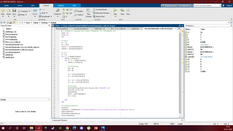
• We start the program with clear all, close all and clc. We are taking a 2 arm robot with arm 1 (l1) of 1m and arm 2 (l2) of 0.5m. The angle between the ground and l1 is theta1 and the angle between l1 and l2 is theta2.
• Since we have to make an animation and not a plot we need multiple values of theta1 and theta2 so we are taking theta1 and theta2 as arrays using the linspace command. We've taken theta1 and theta2 as arrays, but we will need stepwise values of theta1 and theta2 i.e single values and in sequence.
• So the solution for our problem is for loop. I have written ct = 1 i.e counter before the loop, I'll explain the counter later in the explanation. Now taking for i = 1:length(theta1) and THETA1 = theta1(i) and creating another for loop i.e for j = 1: length(theta2) and THETA2 = theta2(j). Here 'i' and 'j' are loop counter variables and 'THETA1' and 'THETA2' are variables and not arrays. So what happens is while plotting the output the program take the 1st value of theta1 and all 5 values of theta2 and then for the 2nd value of theta1 again takes all 2 values of theta2. This process goes on till the program takes the last value of theta1 for all the values of theta2. Now, this happens due to the counter function i.e ct = 1. It is a variable that simply increments (or decrements) by a specific 'step' value in every iteration of a loop. So before ending the loop we take ct = ct+1 to take step by step values of theta1 and theta2. We've taken the coordinates from the first program or we can simply get the coordinates with the help of Fig.1. Just replace theta1 with THETA1 and theta2 with THETA2.
• Now, for plotting, we use the plot function and use linewidth to define the width of the line to 3. And set boundaries to the plot with axis([0 1.5 0 1.5]) which means the plot can be seen only from 0 to 1.5 x-axis and 0 to 1.5 y-axis. The pause function is used to pause the program in between every step and control the speed of the animation, so we get a smooth animation. Now in the next step, we save every frame in an array 'M'.
• Now after ending both the loops we generate a movie i.e Matlab will generate a movie with all the frames in the array 'M'. We use the next step to create an AVI (Audio Video Interleave) file and name the file. Uncompressed AVI means we get the original quality of the file without compression. Next, we are going to open the AVI file and write to the file all the frames captured in the array 'M' and then close the AVI file.
• After saving and running the program first we the output in Matlab figure and then the video is played.
• Honestly, I haven't faced any errors while writing this program as I followed the video lecture.