Week 3 - Solving second order ODEs

OBJECTIVE:

To write a program that solves the equation of motion of a simple pendulum with damping and to will simulate the pendulum motion.

THEORY:

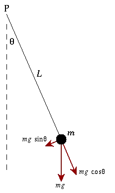
A simple pendulum consists of a ball (point-mass) m hanging from a (massless) string of length L and fixed at a pivot point P. When displaced to an initial angle and released, the pendulum will swing back and forth with periodic motion. By applying Newton's secont law for rotational systems, the equation of motion for the pendulum may be obtained.

PROBLEM STATEMENT:

The above equation is the equation of motion of a simple pendulum with damping.

where,

g = gravity in m/s2,

L = length of the pendulum in m,

m = mass of the ball in kg,

b=damping coefficient.

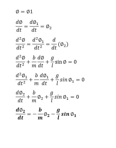
Now for solving the second order ODE we have to convert the second order ODE into number of first order ODE.

Given input data;

L=1 metre,

m=1 kg,

b=0.05.

g=9.81 m/s2.

To simulate the motion between 0-20 sec

angular displacement=0

angular velocity=3 rad/sec at time t=0.

SOLUTION PROCEDURE:

Converting the second order ODE into number of first order ODE

PROCEDURE:

STEP 1 : Import the required modules .Here we have imported math , scipy , odeint ,matplotlib.pyplot modules

STEP 2: Defining a function that will return a value 'dtheta_dt' which has both the first order ODE.

STEP 3: enter input values by assigning the values to several variables

STEP 4:Enter the initial condition . i.e angular displacement=0 , angular velocity =3.

STEP 5:write a code to get n number of time values between 0 to 20 using linspace() command

STEP 6:For solving the ODE use odeint() command

STEP 7:By using plot(),xlabel(),ylabel(),xlim(),ylim(),title() commands plot the graph between time and plot

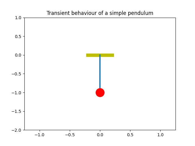
STEP 8:Create animation using a for loop so that we can get X and Y co-ordinates using trignometric functions.

STEP 9:Use file name as filename='pendulum%05d.png'%ct so that there will be no over confusion in running the pictures sequencially.

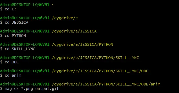
STEP 10:Use this code in cygwin to get a gif

PYTHON CODE:

#importing required modules
import math
from scipy.integrate import odeint 
import numpy as np
import matplotlib.pyplot as plt

#funtion that return dtheta/dt
def model(theta,t,b,g,m,l):
	theta1=theta[0]
	theta2=theta[1]
	dtheta1_dt=theta2
	dtheta2_dt=-(b/m)*theta2-(g/l) *math.sin(theta1)
	dtheta_dt=[dtheta1_dt,dtheta2_dt]
	return dtheta_dt

#input values
b=0.05 #damping coefficient
g=9.81 #gravity (m/s^2)
l=1    #length of the pendulum (m) 
m=1  #mass of the ball (Kg)

#Initial condition
theta0=[0,3]

#Time points
n=500
t=np.linspace(0,20,n)

#soliving ODE
theta=odeint(model,theta0,t,args=(b,g,l,m))

#plotting the graph
plt.plot(t,theta[:,0],'b--',label=r'Angular displacement')
plt.plot(t,theta[:,1],'r-',label=r'Angular velocity')
plt.xlabel('Time(s)')
plt.ylabel('Plot')
plt.title("Damped Hormonic motion of a simple pendulum")
plt.xlim([0,20])
plt.legend(loc='best')
plt.show()

#animation step
ct=1
range=theta[:,0]
for i in range:
	Xo=0
	Yo=0
	X1=Xo+l*math.sin(i)
	Y1=Yo-l*math.cos(i)
    
	
	
	#plotting for animation
	plt.figure()
    #plotting the rigid support through which string of pendulum is attached
	plt.plot([-0.2,0.2],[0,0],linewidth=8,color='y') 
	#plotting string of pendulum
	plt.plot([Xo,X1],[Yo,Y1],linewidth=3)
	#plotting bob of pendulum
	plt.plot(X1,Y1,'o',markersize=20,color='r')
	#plotting dotted vertical line for reference
	plt.xlim([-1.25,1.25])
	plt.ylim([-2,1])
	plt.title('Transient behaviour of a simple pendulum')
	filename='pendulum%05d.png'%ct
	plt.savefig(filename)
	ct=ct+1
	
	

OUTPUT:

ANIMATION:

OBSERVATION:

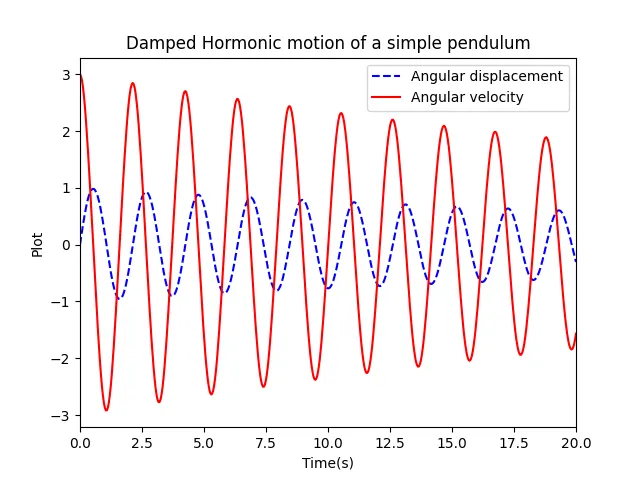
• The reduction in angular displacement and angular velocity is due to the damping coefficienent.
• More the damping coefficient more will be the reduction in the angular velocity and displacement .
• The angular amplitude decreases exponentially over time which depends on the moment of inertia