Week 3 - Solving second order ODEs

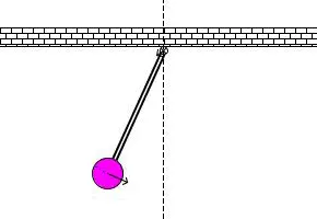
Aim- To write a program that solves the following ODE which represents the equation of motion of a simple pendulum with damping and simulate the motion between 0-20 sec, for angular displacement=0, angular velocity=3 rad/sec at time t=0. When you do this you will get the position of the pendulum as a function of time. Use this information to animate the motion of the pendulum, as shown in the below figure.

Introduction- A simple pendulum is a body suspended from a fixed point so it can swing back and forth under the influence of gravity. Pendulums, like masses on a spring, are examples of Simple Harmonic Motion.

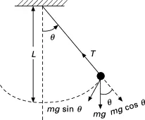
It consists of a small bob of mass 'm' suspended at the end of a thread of length 'L' that is so light as to be considered massless. The period of such a device can be made longer by increasing its length, as measured from the point of suspension to the middle of the bob. A change in the mass of the bob, however, does not affect the period, provided the length is not thereby affected.

Assumptions-

• Gravity remains constant.
• There is negligible friction between the air and the system.
• The pendulum swings in a perfect plane.
• The arm of the pendulum does not bend or compress and is massless.

Governing Equation-

The Ordinary Differential Equation (ODE) that shows the simple pendulum's motion is as follows,

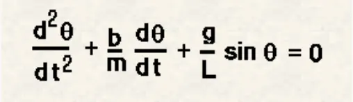
Where,

b = damping coefficient

m = mass of the pendulum bob

L = length of massless string or rod

θ = angle of the pendulum

Input Values-

• L=1 metre,
• m=0.1 kg,
• b=0.05.
• g=9.81 m/s2.

Convert 2nd degree ODE order into first degree ODE=

θ = θ1

dθ/dt = dθ1/dt = θ2

dθ/dt+b*θ/m+g*sinθ1/L

Function's Code-

function [dtheta_dt] = ode_function(t,theta,b,g,l,m)
         
theta1 = theta(1)
theta2 = theta(2)
dtheta1_dt = theta2;
dtheta2_dt = -(b/m)* theta2 -(g/l)*sin(theta1);
dtheta_dt = [dtheta1_dt; dtheta2_dt];
end

Main Program for Simple Pendulum-

clear all
close all
clc



b = 0.05;
g = 9.81;
l = 1;
m = 1;


% Starting Condition
theta_0 = [0;3];


% Time points
t_span = linspace(0,20,300);

% Solving ode
[t , results] = ode45(@(t,theta)ode_function(t,theta,b,g,l,m),t_span, theta_0);
i = 1
figure(1)
grid on
plot(t,results(:,1))
hold on
plot(t,results(:,2))
xlabel('Time')
ylabel('Plot')
legend('CHANGE IN DISPLACEMENT''CHANGE IN ANGULWER VILOCITY')

for i = l:length(t)
x = (sin(results(i,1)));
y = (-cos(results(i,1)));


figure(2)
plot([0, x],[0, y],'-o')
axis ([-1 1 -2 0])
text(0, -1.6, ['Time', num2str(t(i,1))])
M(i) = getframe(gcf);
pause(0.1)
end

movie(M)
videofile = VideoWriter('PENDULUM.avi','Uncompressed AVI');
open(videofile)
writeVideo(videofile,M)
close(videofile)

Results-

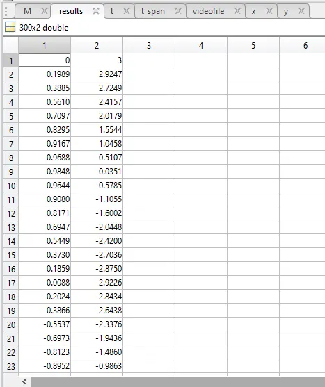
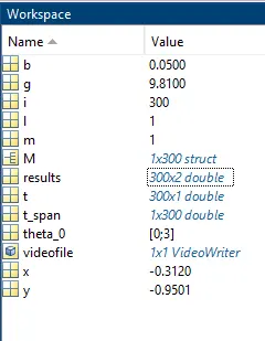
• since we are solving 2 ode's the Results would be a column vector with two columns in which 1st column refers to displacement and 2nd column refers to velocity as shown in the below picture from the workspace

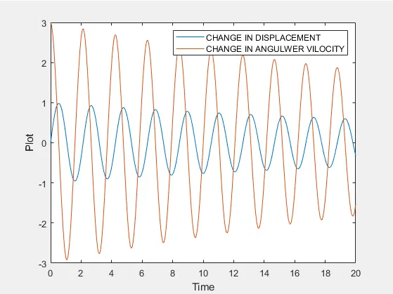
• The graph for the above ODE equation is shown as below :

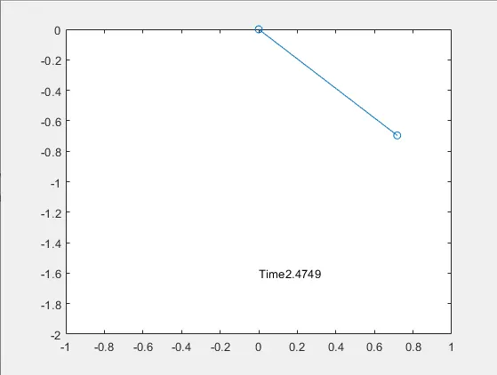
Animation Link is Given Below-

https://youtu.be/vDaNQc1SVPs