Week 3 - Solving second order ODEs

ODE PROGRAM FOR PENDULUM

b=0.05;
g=9.81;
l=1;
m=0.1;

%intial conditions
theta_0=[0;5];

%time [oints
t_span=linspace(0,10,50);

%solve ODE
[t, results]=ode45(@(t,theta) ode_func(t,theta,b,g,l,m),t_span, theta_0);
subplot(2,1,1)
plot(t,results(:,1));
ylabel('plot');
xlabel('time');
subplot(2,1,2)
hold on;
plot(t,results(:,2));
xlabel('time');
ylabel('plot');
grid on;

%animation
X0=0;
Y0=0;
ct=1;
for i=1:length(t)
    X1=l*sin(results(i,1));
    Y1=-l*cos(results(i,1));
    
    figure(2)
    plot([-1 1],[0 0],'linewidth',6,'color','g');
    axis([-2 2 -2 2]);
    line([X0 X1],[Y0,Y1],'linewidth',2,'color','b');
    hold on;
    plot(X0,Y0,'o','markersize',3,'markerfacecolor','y');
      plot(X1,Y1,'o','markersize',20,'markerfacecolor','r');
      title('damping');
      legend('Support','length','fixed','body');
      grid on;
      hold on;
      M(ct)=getframe(gcf);
      ct=ct+1;
end
movie(M)
videofile=VideoWriter('spring.avi','Uncompressed AVI');
open(videofile)
writeVideo(videofile,M)
close(videofile)

FUNCTION CODE

function [dtheta_dt] = ode_func(t,theta,b,g,l,m)
theta1=theta(1)
theta2=theta(2)
dtheta1_dt=theta2;
dtheta2_dt= -(b/m)*theta2-(g/1)*sin(theta1);
dtheta_dt=[dtheta1_dt;dtheta2_dt];
end

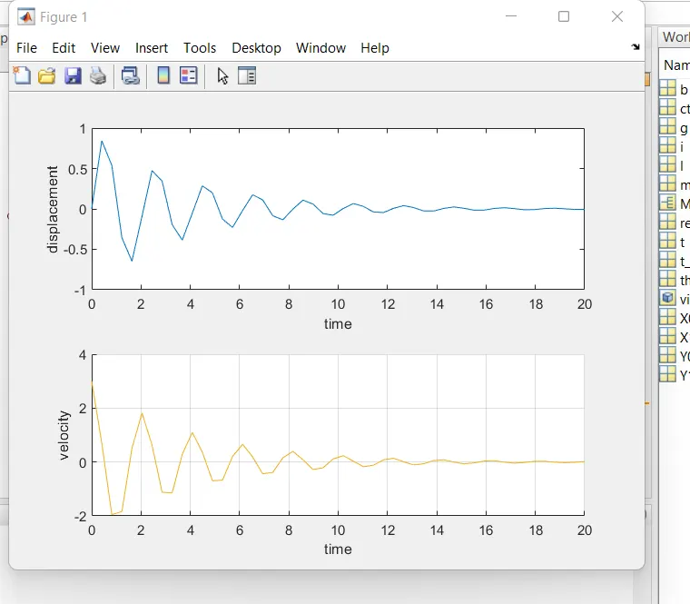
PLOTS

EXPLAINATION

we are solving second ODE of a simple pendulum.

inorder to slove higher order differential equations we are using runge kuta method, where we bring them to first order differential equation.

The seconf ODE quation of pendulum is given as

d^2theta/dt^2+b/m*dtheta/dt+g/l*sin(theta)=0;

where b, g, m, l , are the parameters of the pendulum.

providing intial conditions i.e., displacement and velocity

and time from 0 sec to 20 sec

we now call the ode45 function where the slover computes order differential equation.

this ode function as code for the final equation.

assigning theta values i.e., theta(1) to theta 1

and theta(2) to theta 2

and writing the final equation equation to carry the coding solution

this output will be having two results in the form of matrix.

later this results are plotted

we get the

For the animation part

we use for loops

first we will plot base line by using plot command

and now we will plot fixed support and then to that fixed support we will arrange link having length 1m. to that link we will attach ball having thickness 20.

the animation carries out in the for loop i.e., the condtion given. As the end points of the link are x1 and y1.

for i=1:length(t)
X1=l*sin(results(i,1));
Y1=-l*cos(results(i,1));

this end after all the iterations got completed.

next the animation code is runed inorder to collect the frames of the plotting.

https://drive.google.com/file/d/1eOBkEiI8muQcaIB9NRoB2r5gVm6lIwmx/view?usp=sharing