Project 2 - Rankine cycle Simulator

objectives:

• Create a Rankine Cycle Simulator using OCTAVE/MATLAB.
• Your code should calculate the state points of the Rankine Cycle (any type of your choice) based on user inputs.
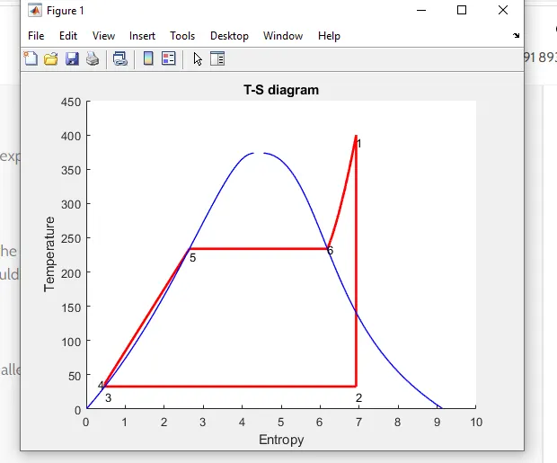
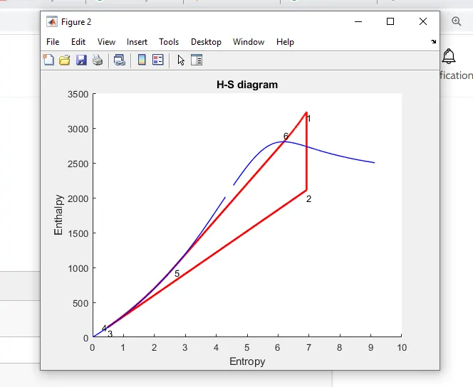
• Then, plot the corresponding T-s and h-s plots for the given set of inputs. Title and axes labels are a must, while legends could be used if necessary.
• The presentation of your code will be taken into consideration while grading. Labelling sections of your code using comments is appreciated.
• Attach a report explaining the working of a rankine cycle simulator and also the research done by you.

Research:

Vapor power plants generate electrical power by using fuels like coal, oil or natural gas. The schematic of a vapor power plant is shown on the left. The entire power plant can be broken down into four major subsystems.

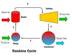
• Subsystem A: Energy conversion from heat to work
• Subsystem B: Energy source and waste removal required to vaporize the water
• Subsystem C: Electric generator
• Subsystem D: Cooling water system

The focus of this chapter is subsystem A. The thermodynamic cycle in subsystem A is called the Rankine cycle. Subsystem A consists of a boiler, turbine, condenser and a pump. Fuel, burned in the boiler, heats the water to generate superheated steam (subsystem B). This steam is used to run the turbine which powers the generator. Electrical energy is generated when the generator windings rotate in a strong magnetic field (subsystem C). After the steam leaves the turbine, it is cooled to its liquid state in the condenser by transferring heat to the cooling water system (subsystem D). The liquid is pressurized by the pump prior to going back to the boiler.

All four components associated with the ideal Rankine cycle are steady-flow devices, and thus all four processes that make up the Rankine cycle can be analyzed as steady-flow process. The kinetic and potential energy changes of water are small relative to the heat and work terms, are thus neglected. Energy analysis of the four components are given below.

Pump (process 1-2): Pump pressurized the liquid water from the condenser prior to going back to the boiler. Assuming no heat transfer with the surroundings, the energy balance in the pupmp.

w_{pump, in} = h₂ - h₁

Boiler (process 2-3): Liquid water enters the boiler and is heated to superheated state in the boiler. The energy balance in the boiler is

q_in = h₃ - h₂

Turbine (process 3-4): Steam from the boiler, which has an elevated temperature and pressure, expands through the turbine to produce work and then is discharged to the condenser with relatively low pressure. Neglecting heat transfer with the surroundings, the energy balance in the turbine.

w_{turbine, out} = h₃ - h₄

Condenser (process 4-1): Steam from the turbine is condensed to liquid water in the condenser. The energy balance in the condensor is

q_out = h₄ - h₁

For the whole cycle, the energy balance can be obtained by summarizing the four energy equations above. It yields,

(q_in- q_out) - (w_{turbine, out} - w_{pump, in}) = 0

The thermal efficiency of the Rankine cycle is determined from

η_th = w_{net ,out}/q_in = 1 - q_out/q_in

where the net work output from the cycle is

w_{net ,out} = w_{turbine, out} - w_{pump, in}

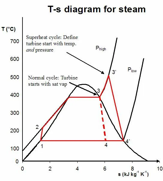
he Rankine cycle is an ideal cycle if water passes through the four components without irreversibilities and pressure drops. The ideal Rankine cycle consists of the following four processes, as shown on the T-s diagram on the left:

• 1-2: Isentropic compression in a pump
• 2-3: Constant pressure heat addition in a boiler
• 3-4: Isentropic expansion in a turbine
• 4-1: Constant pressure heat rejection in a condenser

code:

clear all
close all
clc
% ===================== rankine cycle processes ========================= %
fprintf(' RANKINE CYCLE SIMULATOR')
fprintf('\n1-2 Isentropic expansion in Turbine')
fprintf('\n2-3 Isobaric heat rejection by condensor')
fprintf('\n3-4 Isentropic compression in pump')
fprintf('\n4-1 Isobaric heat addition by boiler \n')
fprintf('\n')
% Given inputs %
P1 = input('pressure at turbine inlet (bar) :');
T1 = input('temperature at turbine inlet (celsius) :');
P2 = input('pressure at condensor (bar) :');
% ==================== Stage -1 (Turbine inlet) ========================= %
% pressure and temperatures are given %
h1 = XSteam('h_pT',P1,T1);
s1 = XSteam('s_pT',P1,T1);
% =================== Stage - 2 (Condenser inlet) ======================= %
% P2 is given % to find h2 %
% h2 = hf2 + x2 (hg2 - hf2) %
% Where x2 = (s2 - sf2)/(sg2 - sf2) %
s2 = s1 ; % Isentropic process
sf2 = XSteam('sL_p',P2);
sg2 = XSteam('sV_p',P2);
x2 = (s2-sf2)/(sg2-sf2);
hf2 = XSteam('hL_p',P2);
hg2 = XSteam('hV_p',P2);
h2 = hf2 + (x2*(hg2 - hf2));
% ======================= Stage - 3 (Pump inlet) ======================== %
P3 = P2; % Isobaric process
% saturated liquid stage %
h3 = XSteam('hL_p',P3);
s3 = XSteam('sL_p',P3);
T3 = XSteam('Tsat_p',P3);
T2 = T3; % for stage - 2
% ======================= Stage - 4 (Boiler inlet)======================= %
s4 = s3; % Isentropic process
P4 = P1; % Isobaric process
h4 = XSteam('h_ps',P4,s4);
% to find T4 % T3/T4 = (P3/P4)^((C-1)/C) %
% Where C = Cp4/Cv4
% Specific heat values %
Cp4 = XSteam('Cp_ps',P4,s4); % constant pressure %
Cv4 = XSteam('Cv_ps',P4,s4); % constant volume %
C = Cp4/Cv4;
T4 = T3/((P3/P4)^((C-1)/C));
% saturated liquid state %
T5 = XSteam('Tsat_p',P1);
s5 = XSteam('sL_p',P1);
h5 = XSteam('hL_p',P1);
% saturated vapour state %
T6 = T5;
s6 = XSteam('sV_p',P1);
h6 = XSteam('hV_p',P1);
% Calculation of work (KJ/Kg) %
Wt = h1 - h2; % Turbine work
Wp = h4 - h3; % Pump work
W = Wt - Wp; % Net work Output
% Calculation of heats %
Qin = h1 - h4; % heat addition in boiler
Qout = h2 - h3; % heat removed in condeser
% Thermal Efficiency (%) %
nTherm = (W/Qin)*100;
% Steam rate (Kg/KWh) %
SSC =3600/W;
% Back work ratio %
BWR = Wp/Wt;
% ============================== Plotting =============================== %
% plotting T-S diagram %
figure(1)
hold on
title('T-S diagram')
plot([s1 s2],[T1 T2],'linewidth',2,'color','r')
plot([s2 s3],[T2 T3],'linewidth',2,'color','r')
plot([s3 s4],[T3 T4],'linewidth',2,'color','r')
plot([s4 s5],[T4 T5],'linewidth',2,'color','r')
plot([s5 s6],[T5 T6],'linewidth',2,'color','r')
s_1 = linspace(s6,s1,500);
for j = 1:length(s_1);
 t_1(j) = XSteam('T_ps',P1,s_1(j));
end
plot(s_1,t_1,'linewidth',2,'color','r')
xlabel('Entropy')
ylabel('Temperature')
% plot saturation curve %
T = linspace(1,T1,500);
for i = 1:length(T);
 h_l(i) = XSteam('hL_T',T(i));
 h_v(i) = XSteam('hV_T',T(i));
 s_l(i) = XSteam('sL_T',T(i));
 s_v(i) = XSteam('sV_T',T(i));
end
plot(s_l,T,'linewidth',1,'color','b')
plot(s_v,T,'linewidth',1,'color','b')
% annotations %
text(s1,T1,'1','verticalalignment','top')
text(s2,T2,'2','verticalalignment','cap')
text(s3,T3,'3','verticalalignment','cap')
text(s4,T4,'4','horizontalalignment','right')
text(s5,T5,'5','verticalalignment','top')
text(s6,T6,'6','horizontalalignment','left')
% plotting H-S diagram %
figure(2)
hold on
title('H-S diagram')
plot([s1 s2],[h1 h2],'linewidth',2,'color','r')
plot([s2 s3],[h2 h3],'linewidth',2,'color','r')
plot([s3 s4],[h3 h4],'linewidth',2,'color','r')
h_4 = linspace(h4,h5,500);
for k = 1:length(h_4)
 s_4(k) = XSteam('s_ph',P1,h_4(k));
end
h_6 = linspace(h6,h1,500);
for m = 1:length(h_6)
 s_6(m) = XSteam('s_ph',P1,h_6(m));
end
plot(s_4,h_4,'linewidth',2,'color','r')
plot([s5 s6],[h5 h6],'linewidth',2,'color','r')
plot(s_6,h_6,'linewidth',2,'color','r')
xlabel('Entropy')
ylabel('Enthalpy')
% plot saturation curve %
plot(s_l,h_l,'linewidth',1,'color','b')
plot(s_v,h_v,'linewidth',1,'color','b')
% annotations %
text(s1,h1,'1','verticalalignment','top')
text(s2,h2,'2','verticalalignment','cap')
text(s3,h3,'3','verticalalignment','top')
text(s4,h4,'4','horizontalalignment','right')
text(s5,h5,'5','verticalalignment','top')
text(s6,h6,'6','verticalalignment','bottom')
% Results window %
fprintf('\n RESULTS')
fprintf('\n >>>At state point 1 :')
fprintf('\n P1 is : %f Bar',P1)
fprintf('\n T1 is : %f Deg celcius',T1)
fprintf('\n H1 is : %f KJ/Kg',h1)
fprintf('\n S1 is : %f KJ/KgK',s1)
fprintf('\n')
fprintf('\n >>>At state point 2 :')
fprintf('\n P2 is : %f Bar',P2)
fprintf('\n T2 is : %f Deg celcius',T2)
fprintf('\n H2 is : %f KJ/Kg',h2)
fprintf('\n S2 is : %f KJ/KgK',s2)
fprintf('\n')
fprintf('\n >>>At state point 3 :')
fprintf('\n P3 is : %f Bar',P3)
fprintf('\n T3 is : %f Deg celcius',T3)
fprintf('\n H3 is : %f KJ/Kg',h3)
fprintf('\n S3 is : %f KJ/KgK',s3)
fprintf('\n')
fprintf('\n >>>At state point 4 :')
fprintf('\n P4 is : %f Bar',P4)
fprintf('\n T4 is : %f Deg celcius',T4)
fprintf('\n H4 is : %f KJ/Kg',h4)
fprintf('\n S4 is : %f KJ/KgK',s4)
fprintf('\n')
fprintf('\n Turbine work : %f KJ/Kg',Wt)
fprintf('\n Pump work : %f KJ/Kg',Wp)
fprintf('\n Net work output : %f KJ/Kg',W)
fprintf('\n Thermal efficiency : %f percent',nTherm)
fprintf('\n SSC : %f Kg/KWh',SSC)
fprintf('\n Back work ratio : %f',BWR)
fprintf('\n')

code explanation

The program is started with the clear all, close all and clc to clear the
workspace, command window and plots.

• Information about the cycle and their processes are mentioned using the
'fprintf' command.
• Input variables P1, T1 and P2 are given by 'input' command whose values are
entered in command window while executing the program.

where

p1= initial turbine pressure

T1= turbine inlet intial temperature

P2= turbine outlet pressure

• The data for the properties of steam and water are extracted from the
XSteam.m file.this xsteam data file as the data that is required to find enthaply, entropy, specific heat ate given temperature and pressure.

• At state 1, the values for the enthalpy and entropy are extracted as a function
of temperature and pressure.

h1 = XSteam('h_pT',P1,T1);
s1 = XSteam('s_pT',P1,T1);

here h1 is extracted by xsteam data file at p1 and t1 pessure and teperatures.

s1 aslo at p1 and t1

inorder to plot the curve we will use for loop where the values range from s1 to s6 have 500values betwwen them having the condition

for j = 1:length(s_1);
t_1(j) = XSteam('T_ps',P1,s_1(j));

that means for each and every value of j t_1 carries values of temperature and pressure .

this is looped upto s6

similary it continues with the same logic for the saturation curve.

• for other states the enthalpy is found out using the formulas that are gievn above .

but for us inorder to find the h2 we will first find,

hf2 where

hf2=enthalpy of liquid at pressure 2.

x2= entropy at state 2 - fluid entropy at state 2/gas entropy - fulid entropy at state 2

similarly

hg2(enthalpy of gas at state 2 ) is drewan from xsteam data file by command hg2 = XSteam('hV_p',P2);

similarly we need to find other quantites in the same way by relating and finding values corresponding quantities.

% =================== Stage - 2 (Condenser inlet) ======================= %
% P2 is given % to find h2 %
% h2 = hf2 + x2 (hg2 - hf2) %
% Where x2 = (s2 - sf2)/(sg2 - sf2) %
s2 = s1 ; % Isentropic process
sf2 = XSteam('sL_p',P2);
sg2 = XSteam('sV_p',P2);
x2 = (s2-sf2)/(sg2-sf2);
hf2 = XSteam('hL_p',P2);
hg2 = XSteam('hV_p',P2);
h2 = hf2 + (x2*(hg2 - hf2));
% ======================= Stage - 3 (Pump inlet) ======================== %
P3 = P2; % Isobaric process
% saturated liquid stage %
h3 = XSteam('hL_p',P3);
s3 = XSteam('sL_p',P3);
T3 = XSteam('Tsat_p',P3);
T2 = T3; % for stage - 2
% ======================= Stage - 4 (Boiler inlet)======================= %
s4 = s3; % Isentropic process
P4 = P1; % Isobaric process
h4 = XSteam('h_ps',P4,s4);
% to find T4 % T3/T4 = (P3/P4)^((C-1)/C) %
% Where C = Cp4/Cv4
% Specific heat values %
Cp4 = XSteam('Cp_ps',P4,s4); % constant pressure %
Cv4 = XSteam('Cv_ps',P4,s4); % constant volume %
C = Cp4/Cv4;
T4 = T3/((P3/P4)^((C-1)/C))

• The formula for calculating the unknown state values of temperature,
pressure, enthalpy and entropy are calculated from the basic formulas from
reference book.

• After calculating the values at all states, work done and heat transfer are
calculated.

• The efficiency, specific steam consumption and back work ratio are also
calculate using the above formulas.

• The saturation curve is plotted, temperature range is defined using the
'linspace' command and values of enthalpy and entropy are calculated at
each temperature point. These values are used to draw the saturation curves
in the h-s and t-s diagrams.

• Now the cycle is plotted over the saturation curve and annotations for each
process are specified using the 'text' command.

• All the results of the Rankine cycle are plotted using the 'fprintf' command.

output

RANKINE CYCLE SIMULATOR
1-2 Isentropic expansion in Turbine
2-3 Isobaric heat rejection by condensor
3-4 Isentropic compression in pump
4-1 Isobaric heat addition by boiler

pressure at turbine inlet (bar) :30
temperature at turbine inlet (celsius) :400
pressure at condensor (bar) :0.05

RESULTS
>>>At state point 1 :
P1 is : 30.000000 Bar
T1 is : 400.000000 Deg celcius
H1 is : 3231.571027 KJ/Kg
S1 is : 6.923259 KJ/KgK

>>>At state point 2 :
P2 is : 0.050000 Bar
T2 is : 32.875490 Deg celcius
H2 is : 2110.708212 KJ/Kg
S2 is : 6.923259 KJ/KgK

>>>At state point 3 :
P3 is : 0.050000 Bar
T3 is : 32.875490 Deg celcius
H3 is : 137.765119 KJ/Kg
S3 is : 0.476254 KJ/KgK

>>>At state point 4 :
P4 is : 30.000000 Bar
T4 is : 36.935287 Deg celcius
H4 is : 140.762226 KJ/Kg
S4 is : 0.476254 KJ/KgK

Turbine work : 1120.862815 KJ/Kg
Pump work : 2.997107 KJ/Kg
Net work output : 1117.865709 KJ/Kg
Thermal efficiency : 36.167417 percent
SSC : 3.220423 Kg/KWh
Back work ratio : 0.002674

plot diagrams: