Challenge

Week 3 - Solving second order ODEs

VVinayak G Kurup23 Dec 2021

MATLAB

Aim

To solve the second order differential equation using MATLAB which mathematical of motion of pendulum

and to create an animation for that equation.

Objective

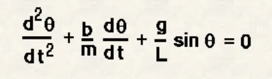
To write a program thet solves the following ODE which represents the equation of motion of a simple

pendulum with damping and create an animayed video of output obtained by solving this ODE.

Theory

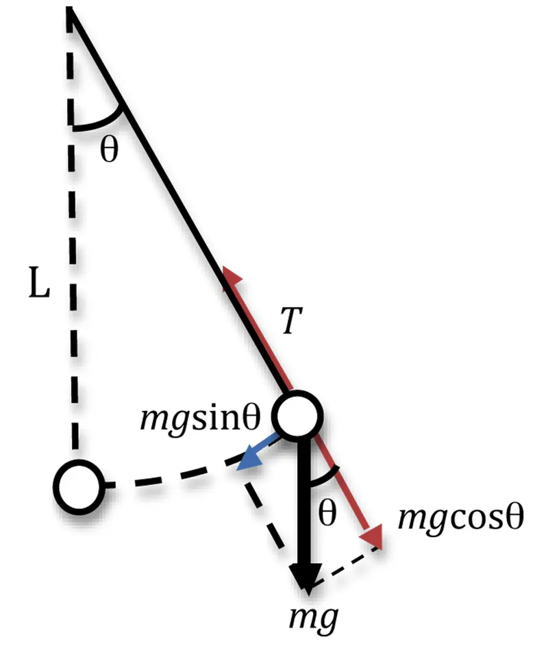
The motion of simple pendulum is a basic classical example of simple harmonic motion, consisting of a

small bob and a massless string. Movement of th pendulum depends on Newtons's second law.when this

law is written down,a second-order Ordinary Different Equation is formed thet described the postion of

the pendulum w.r.t time.

Simple Pendulum

Equation of motion is :

In the above equation,

1. g = gravity in m/s^2

2. L = length of the pendulum in meter.

3. m = mass of the ball in kg.

4. b = damping cofficient.

Since the given function is in the second-order differential equation w will convert it into first order to

solve the ODE.

Let

θ = θ1

dθ/dt = θ2

dθ^2/dt^2 = dθ2/dt

Input

1. L = 1 meter

2. m = 1kg

3. b = 0.05

4. g = 9.81m/s^2

5. Time span = 0-20s

6. Angular displacement = 0

7. Angular velocity = 3 rad/sec2 at time t =0

Main Code

clear all
close all
clc

b=0.05;
g=9.81;
l=1;
m=1;

% inital condition
theta_0 = [0;5];

% time points
t_span = linspace(0,20,100);

% solve ODE
[t, results] = ode45(@(t,theta) ode_func(t, theta, b,g,l,m),t_span, theta_0); 

plot(t,results(:,1))
hold on
plot(t,results(:,2))
ylabel('Plot')
xlabel('time')
legend('Displacement (m)','velocity (m/s^2)');
saveas(figure(1),'SHM.jpg');
theta = results(:,1);
i = 1;

for j = 1:length(theta)
    Theta = theta(j);
    
    % initial points
    x0 = 0;
    y0 = 0;
    
    % movements of pendulum
    
    x1 = 1*sin(Theta);
    y1 = -1*cos(Theta);
    
    figure (2);
    
    % ploting string
    
    plot([x0 x1],[y0 y1],'color','g');
    hold on
    
    % ploting the pendulum bob
    
    plot(x1,y1,'o','markersize',10,'color','r','markerfacecolor','r');
    hold off
    
    axis([-1.2 1.2 -1.2 1.2]);
    pause(0.001);
    M(i) = getframe(gcf);
    i = i+1;
end

movie(M);
videofile = VideoWriter('pendulum1.avi','Uncompressed avi')
open(videofile)
writeVideo(videofile,M)
close(videofile);

1. In the above program, the fixed parameters are length, mass,damping coefficient and acceleration due

to gravity.

2. Time and angle are given as the initial condition.

3. In the t_span command.100 values are taken in between 0 to 20 time period

4. Using the ode45 command ODE function is introduced.

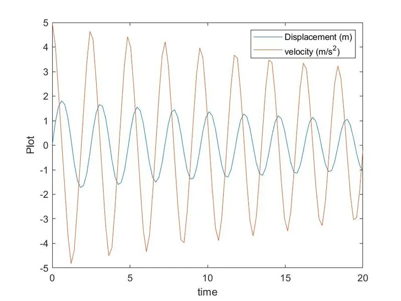
5. Using the plot command velocity and displacement are plotted in the y-axis aganist time on the

x-axis

6. Using the loop command the mass at various points and various times are marked in the graph and are

plotted.

7. using the movie command the plot is saved as an uncompressed.avi file.

Function Code:- ode_func

function [dtheta_dt] = ode_func(t,theta,b,g,l,m)

    theta1 = theta(1);
    theta2 = theta(2);
    dtheta1_dt = theta2;
    dtheta2_dt = -(b/m)*theta2 - (g/l)*sin(theta1);
    dtheta_dt = [dtheta1_dt; dtheta2_dt];
end

1. In this function program the second order ODE is simplified to the first_order ODE by introducing the

the term theta 1 and theta2

2. Then theta1 & theta2 are differentiated and the dtheta_dt gives a column matrix.\

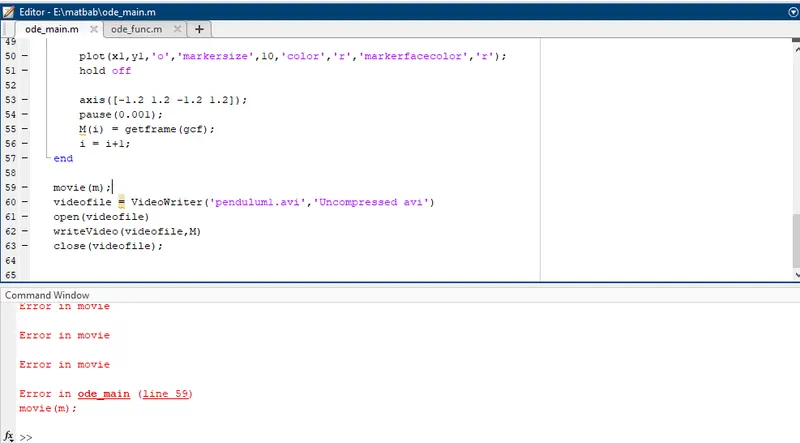
Error