Week 3 - Solving second order ODEs

OBJECTIVE:

To understand the relationship between displacement & velocity of the pendulum with time variable by solving the second order differential equations and also show the simulation of the simple pendulum in matlab.

SOLUTION PROCEDURE:

We will be able to the solve second order ODE with the help of ode45 function. Firstly we have to breakdown the second ODE to two first ODE to easily solve for the desired outputs

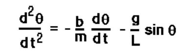
With these equations we can modify the above equation like below

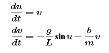
Hence by solving two first ODE we will be able to determine the displacement & velocity of

Pendulum.

We have the below code structured in the following steps

• The following inputs are assumed for this calculation
  1. Length of the string
  2. Mass of the string (negligible so zero)
  3. Mass at the end of spring
  4. Damping coefficient
  5. Initial condition (angle & velocity of the pendulum)
• Function definition with the two first order ODE inside the function block & returning the displacement & velocity
• Solving for the displacement & velocity with the help of odeint & defined function for the number of time intervals required.
• Creating the multiple images of the pendulum with the help of the angular displacement obtained in the previous step.
• Combining the multiple image into one array then converting the images into video file with writevideo command.

Syntax of ODE45:

[t,y] = ode45(odefun,tspan,y0)

where,

          odefun is the functions which is to solved to get the final values of y 

          tspan is the span of the time in which the function has to be differentiated 

          y0 is the initial conditions for the y variable

          t & y are the outputs which will show the y value at the corresponding to the time period

CODE REFERENCE:

MAIN PROGRAM:

clear all
close all
clc

%inputs
%damping coefficient
b=0.05;
%mass of the object
m=1;
%length of the string
l=1;
%acceleration due to gravity 
g=9.8;

%initial condition
% initial angular velocity is 3 rad/s
% initial angular displacement is 0 rad
theta_0=[0;3];

%Array for time
t_span=linspace(0,20,200);

%Solve ODE
[t, results]=ode45(@(t,theta) ode_func(t,theta,b,g,m,l),t_span,theta_0);
fig1=figure(1)
plot(t, results(:,1),"DisplayName",'Displacement')
hold on
plot(t,results(:,2),'DisplayName','Velocity')
xlabel('Time in seconds')
ylabel('Displacement & Velocity')
legend
hold off
%String initial conditions
x0=0;
y0=0;
ct=1;
%Creating the image of pendulum
for i = 1:length(results(:,1))
    angle=results(i,1);
    x1=l*sin(angle);
    y1=-l*cos(angle);
    fig=figure(2)
    plot([-0.25 0.25],[0 0],'LineWidth',1,'Color',[0 0 0])
    hold on
    plot([x0 x1],[y0 y1],'LineWidth',2,'Color','b')
    plot(x1,y1,'Color','r','Marker','o','MarkerSize',15,'MarkerFaceColor','auto')
    axis([-1.5 1.5 -1.5 0.5])
    hold off
    %Array to hold images
    M(ct)=getframe(fig);
    ct=ct+1
end

%Video file creation
videofile=VideoWriter('Pendulum','Uncompressed AVI');
open(videofile)
writeVideo(videofile,M)
close(videofile)

ODE FUNCTION:

function [d_theta]=ode_func(t,theta,b,g,m,l)
    theta1=theta(1);
    theta2=theta(2);
    d_theta1=theta2;
    d_theta2=((-b/m)*theta2)-((g/l)*sin(theta1));
    d_theta=[d_theta1;d_theta2];
end

RESULTS:

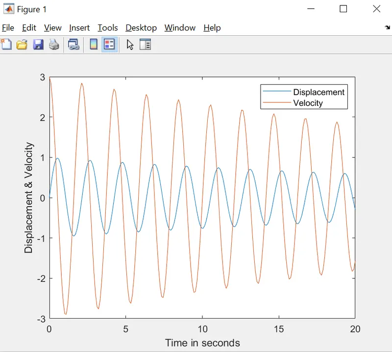
We have the plot which describes the displacement & velocity with respect to time

 

Animation file link for the motion of the pendulum

https://youtu.be/31uOBGeZlik