Week 3 - Solving second order ODEs
2)To wrtite a matlab program to stimulate pendulum motions;


When we bring all the terms to the left-hand side, our model equation becomes

L=1 metre,m=1 kg,b=0.05,g=9.81 m/s2.
3)Understanding ode45 command in Matlab.
%we have
%differntial equation of simple pendulum
%(d^2_theta/dt^2)+(b/m)d_theta/dt+(g/l)
%dtheta1_dt=theta2;
%dtheta2_dt= -(b/m)*theta2-(g/l)*sind(theta1);
%specific gravity
g=9081; %(m/s^2)
%length of the string
l=1; %m
%initial angular disp=0;initial angular vel=3rad/sec
theta_0=[0;3];
%clc
%close all
%clear all


%we have
%differntial equation of simple pendulum
%(d^2_theta/dt^2)+(b/m)d_theta/dt+(g/l)

%dtheta1_dt=theta2;
%dtheta2_dt= -(b/m)*theta2-(g/l)*sind(theta1);


%theta=displacement

%damping coefficient
b=0.05;

%mass
m=0.1; %kg

%specific gravity
g=9081; %(m/s^2)
%length of the string
l=1; %m

%initial condition

%initial angular disp=0;initial angular vel=3rad/sec
theta_0=[0;3];

%time span
t_span=linspace(0,20,500);

%second order differential equation solving
[t,results]=ode45(@(t,theta) fode_func(t,theta,b,m,g,l),t_span,theta_0);

%plotting time vs results

plot(t,results(:,1))
hold on
plot(t,results(:,2))


title("numerical solution of second order differential equation")

xlabel('time(s)')
ylabel('theta(displacement)')

grid on ;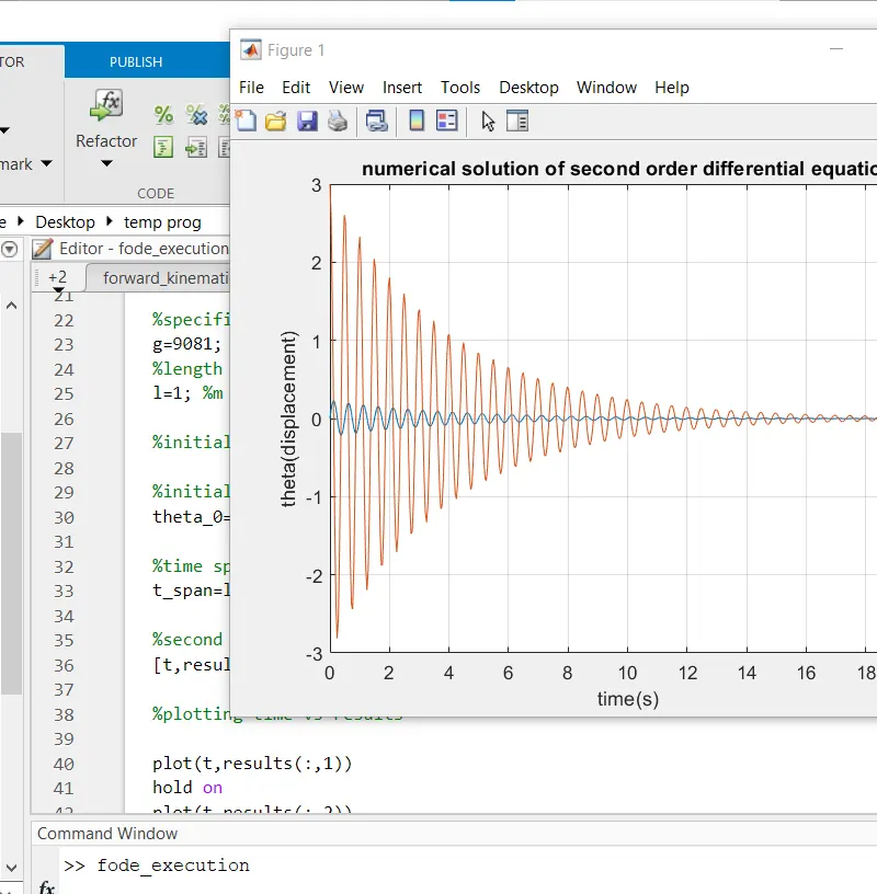
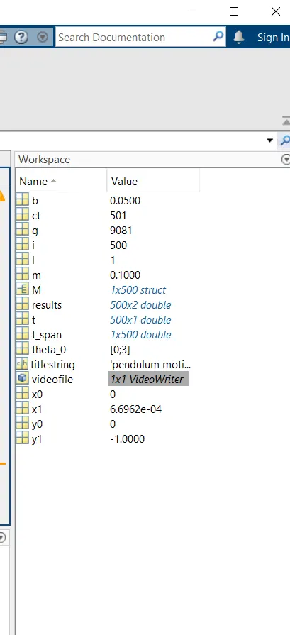
Errors occured and faced duiring execution
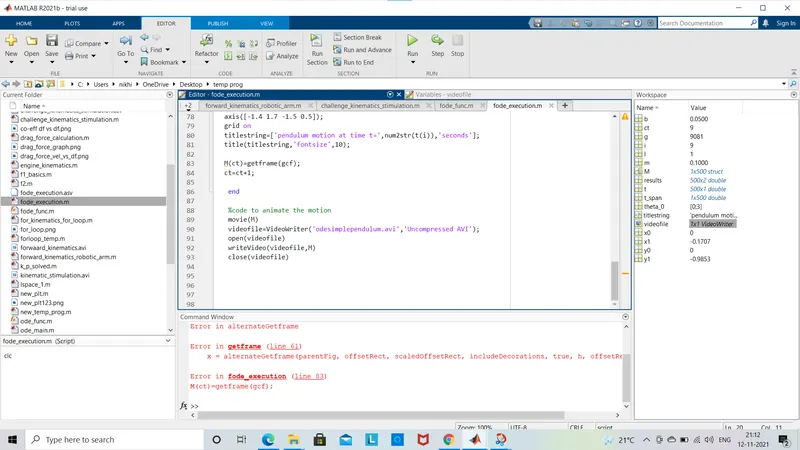
Stimulation of simple pendulum of position of ball wrt time and clear the errors and execution
%stimulation
% below code will help to animate the motion of simple pendulum
figure(2)
ct=1;
for i=1:length(results(:,1))
x0=0;
y0=0;
plot([-1 1],[0 0],'linewidth',4,'color','k');
hold on
%position of ball
x1=l*sin((results(i,1)));
y1=-l*cos((results(i,1)));
%plotting length of pendulum
plot([x0 ,x1],[y0 y1],'LineWidth',2,'Color','r');
%plotting length of fixxed end
plot(x0,y0,'-s','MarkerEdgeColor','k','MarkerFaceColor','b','MarkerSize',10);
%plotting of ball
plot(x1,y1,'-o','MarkerEdgeColor','k','MarkerFaceColor','c','MarkerSize',20);
hold off
axis([-1.4 1.7 -1.5 0.5]);
grid on
titlestring=['pendulum motion at time t=',num2str(t(i)),'seconds'];
title(titlestring,'fontsize',10);
%code to animate the motion
movie(M)
videofile=VideoWriter('odesimplependulum.avi','Uncompressed AVI');
open(videofile)
writeVideo(videofile,M)
close(videofile)
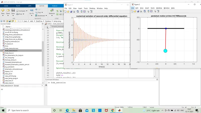
Code wrt function used to solve ode convertiong sode to fode
%ODE FUNCTION
function[dtheta_dt]=fode_func(t,theta,b,m,g,l);
theta1=theta(1);
theta2=theta(2);
%differentiation of above theta1 & 2
dtheta1_dt=theta2;
dtheta2_dt= -(b/m)*theta2-(g/l)*sind(theta1);
dtheta_dt=[dtheta1_dt;dtheta2_dt];
Yopu tube link for the stimulation of simple pendulum animated plot
1)Ode has been solved using ode45 in matlab
2)Motion of simple pendulum as been animated
3)From the above example we understand the concept of damping systems using second laws of Newton.