Air standard cycle

Aim:
Matlab program to plot pv diagram and calculate thermal effeciency of an otto cycle.

Objective:
*To plot the pressure and volume characteristics of an otto cycle.
*To find thermal effeciency of the otto cycle
*To understand the ideal gas laws.
*Understand the natural of curve during the corresponding isentropic process
*Analyse the change in vol with respect to crank angle.

Theory:

OTTO CYCLE

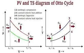
An Otto cycle is an idealized thermodynamic cycle that describes the functioning of a typical spark ignition piston engine. It is the thermodynamic cycle most commonly found in automobile engines.^[1]

The Otto cycle is a description of what happens to a mass of gas as it is subjected to changes of pressure, temperature, volume, addition of heat, and removal of heat. The mass of gas that is subjected to those changes is called the system. The system, in this case, is defined to be the fluid (gas) within the cylinder. By describing the changes that take place within the system, it will also describe in inverse, the system's effect on the environment. In the case of the Otto cycle, the effect will be to produce enough net work from the system so as to propel an automobile and its occupants in the environment.

The Otto cycle is constructed from:

Top and bottom of the loop: a pair of quasi-parallel and isentropic processes (frictionless, adiabatic reversible).

Left and right sides of the loop: a pair of parallel isochoric processes (constant volume).

The isentropic process of compression or expansion implies that there will be no inefficiency (loss of mechanical energy), and there be no transfer of heat into or out of the system during that process. The cylinder and piston are assumed to be impermeable to heat during that time. Work is performed on the system during the lower isentropic compression process. Heat flows into the Otto cycle through the left pressurizing process and some of it flows back out through the right depressurizing process. The summation of the work added to the system plus the heat added minus the heat removed yields the net mechanical work generated by the system.

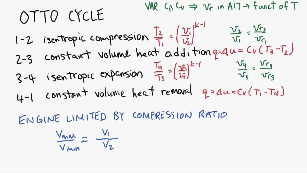
PISTON TERMINOLOGIES

MATLAB PROGRAM

clear all
close all
clc
%INITIALLY GIVEN VALUES 
%STATE VARIABLES
p1=101325;%PRESURRE 1
t1=500;%TEMP 1
gamma=1.4;%SPECIFIC HEAT RATIO
t3=2300;%TEMP3

bore=0.1; 
stroke=0.1;
conn_rod=0.15;
cr=12;

v_s=(pi/4)*bore^2*stroke;%SWEPT VOLUME
v_c=v_s/(cr-1);%CLEARENCE VOL
%STATE 1
v1=v_s+v_c;
v2=v_c;
p2=p1*(v1/v2)^gamma;
t2=(p2*v2*t1)/(p1*v1);

%STATE 2
v_compression=p_k(bore,stroke,conn_rod,cr,180,0);
const_c=p1*v1^gamma;
p_compression=const_c./v_compression.^gamma;
%STATE 3
v3=v2;
p3=(p2*v2*t3)/(v3*t2);

v_expanssion=p_k(bore,stroke,conn_rod,cr,0,180);
const_c=p3*v3^gamma;
p_expanssion=const_c./v_expanssion.^gamma;

%STATE 4
v4=v1;
p4=(p3)*(v3/v4)^gamma;

%thermal efficiency
thermal_efficiency=1-1/cr^(gamma-1);


%plot
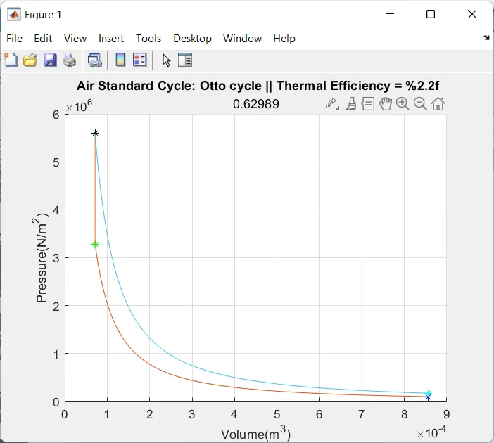
figure(1)
hold on
grid on
colour = [rand rand rand];
plot(v1,p1,'*','color','b') 
 plot(v_compression,p_compression);
plot(v2,p2,'*','color','g')
plot([v2 v3],[p2 p3],'color',colour)
plot(v3,p3,'*','color','k')
plot(v_expanssion,p_expanssion);
plot(v4,p4,'*','color','cyan')
% plot([v4 v1],[p4 p1],'color',colour)
title(" Air Standard Cycle: Otto cycle || Thermal Efficiency = %2.2f",thermal_efficiency);
% legend("Initial state","Isentropic compression","Before heat addition","Isochoric heat addition","After heat addition","Isentropic expansion","Heat rejection starts","Isochoric heat rejection")
xlabel('Volume(m^3)')
ylabel('Pressure(N/m^2)')



%FUNCTION
function [v]=p_k(bore,stroke,conn_rod,cr,start_crank,end_crank);
%ERRORS
% theta=linspace(start_crank,end_crank,180); %180 instead of 100
% v_s=(pi/4)*bore^2*stroke;
% v_c=v_s/(cr-1);
% a=stroke/2;
% r=con_rod/a;
% term1=0.5*(cr-1);
% term2=r+1-cosd(theta);
% term3=(r^2-sind(theta).^2).^0.5;
% %v=(1+term1*term2-term3)*v_c; -> This is incorrect
% v=(1+term1*(term2-term3))*v_c;
%we have=v=1+0.5(rc-1)*[r+1-cosd(theta)-(r^2-sind(theta)^2)^0.5]*v_c

theta=linspace(start_crank,end_crank,180);
v_s=(pi/4)*bore^2*stroke;
v_c=v_s/(cr-1);
a=stroke/2;%CRANK PIN RADIUS
r=conn_rod/a;
%v/v_c=0.5*(cr-1)*[r+1-cosd(theta)-(r^2-sind(theta).^2)^.0.5];
term1=0.5*(cr-1);
term2=r+1-cosd(theta);
term3=(r^2-sind(theta).^2).^0.5;
v=(1+term1*(term2-term3))*v_c;
end

Conclusion:
*Therefore we can calculate temperature at any point for given pressure and volume.
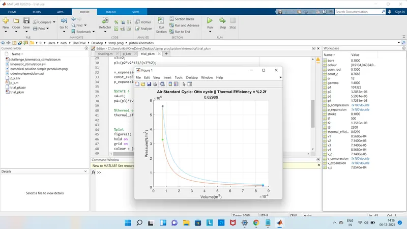
*We can also confirm the Ideal Gas law from the obtained plot.
We can also change the effeciency of the cycle by changing the input parameters.
*We could analize the relationship between the curve characteristics and engine geometry.