CurveFitting using Matlab

Aim:To write a Curve fitting Matlab Programme to perform best fit fotr the given dataset:

Objectives:
* Write code to fit a linear and cubic polynomial for the Cp data.
* Plot the linear and cubic fit curves along with the raw data points. Title and axes labels are a must, legends could be shown if necessary.
* Write a code to show splitwise method.
* Explain the parameters used to measure the fitness characteristics for both the curves.

Body of the content:
Theory:-
Curve fitting is the process of constructing a curve, or mathematical function, that has the best fit to a series of data points,possibly subject to constraints. Curve fitting can involve either interpolation, where an exact fit to the data is required, or smoothing, in which a "smooth" function is constructed that approximately fits the data. A related topic is regression analysis, which focuses more on questions of statistical inference such as how much uncertainty is present in a curve that is fit to data observed with random errors. Fitted curves can be used as an aid for data visualization, to infer values of a function where no data are available,and to summarize the relationships among two or more variables. Extrapolation refers to the use of a fitted curve beyond the range of the observed data, and is subject to a degree of uncertaintysince it may reflect the method used to construct the curve as much as it reflects the observed data.

Fitting of a curve:-

The first degree polynomial equation

is a line with slope a. A line will connect any two points, so a first degree polynomial equation is an exact fit through any two points with distinct x coordinates.

If the order of the equation is increased to a second degree polynomial, the following results:

This will exactly fit a simple curve to three points.

If the order of the equation is increased to a third degree polynomial, the following is obtained:

Parameters used to measure the fitness of the curve:-

• Sum of squared errors:-

In statistics, the residual sum of squares (RSS), also known as the sum of squared residuals (SSR) or the sum of squared estimate of errors (SSE), is the sum of the squares of residuals (deviations predicted from actual empirical values of data). It is a measure of the discrepancy between the data and an estimation model, such as a linear regression. A small RSS indicates a tight fit of the model to the data. It is used as an optimality criterion in parameter selection and model selection.

In a model with a single explanatory variable, RSS is given by:

• R_squared

In statistics, the coefficient of determination, also spelled coëfficient, denoted R² or r² and pronounced "R squared", is the proportion of the variation in the dependent variable that is predictable from the independent variable.

	=	coefficient of determination
	=	sum of squares of residuals
	=	total sum of squares

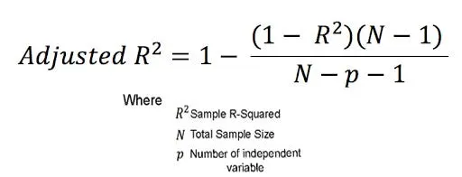
• Adjusted R_square :-Adjusted R-squared is a modified version of R-squared that has been adjusted for the number of predictors in the model. The adjusted R-squared increases when the new term improves the model more than would be expected by chance. It decreases when a predictor improves the model by less than expected.
  
• RSME(root mean square Error)
  The root-mean-square deviation (RMSD) or root-mean-square error (RMSE) is a frequently used measure of the differences between values (sample or population values) predicted by a model or an estimator and the values observed. The RMSD represents the square root of the second sample moment of the differences between predicted values and observed values or the quadratic mean of these differences. These deviations are called residuals when the calculations are performed over the data sample that was used for estimation and are called errors.
  
• Matlab Programme

• clc
  clear all
  close all

  %loading the data to matlab
  cp_data=load('data123');
  %first column temperature
  temprature=cp_data(:,1);
  %second column specific heat
  cp=cp_data(:,2);

  %split wise method into two parts

  
  temperature1=temprature(1:1600,1);
  cp1=cp(1:1600,1);

  temperature2=temprature(1601:3200,1);
  cp2=cp(1601:3200,1);
  %considering first order of polynomial eqn y=ax+bx
  %polyfit used to determine coefficients of a,b

  coefficient1=polyfit(temperature1,cp1,1);
  coefficient2=polyfit(temperature2,cp2,1);

  %polyval used to determine the predicted value of cp
  predicted_cp1=polyval(coefficient1,temperature1);
  predicted_cp2=polyval(coefficient2,temperature2);

  %ploting original data and predicted data curve
  plot(temprature,cp,'LineWidth',3,'Color','b');
  hold on
  plot(temperature1,predicted_cp1,'LineWidth',3,'Color','r');
  hold on
  plot(temperature2,predicted_cp2,'LineWidth',3,'Color','g');
  legend('original database','predicted curve fit')
  title(' linear curve fit')
  
  xlabel('temperature[k]')
  ylabel('specific heat[KJ/KMOL-K]')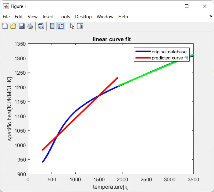

  

• Cubic curve fit

• clc
  clear all
  close all

  %loading the data to matlab
  cp_data=load('data123');
  %first column temperature
  temprature=cp_data(:,1);
  %second column specific heat
  cp=cp_data(:,2);

  %split wise method into two parts

  
  temperature1=temprature(1:1600,1);
  cp1=cp(1:1600,1);

  temperature2=temprature(1601:3200,1);
  cp2=cp(1601:3200,1);
  %considering third order of polynomial eqn y=ax^3+bx^2+cx+d
  %polyfit used to determine coefficients of a,b

  coefficient1=polyfit(temperature1,cp1,3);
  coefficient2=polyfit(temperature2,cp2,3);

  %polyval used to determine the predicted value of cp
  predicted_cp1=polyval(coefficient1,temperature1);
  predicted_cp2=polyval(coefficient2,temperature2);

  %ploting original data and predicted data curve
  plot(temprature,cp,'LineWidth',3,'Color','b');
  hold on
  plot(temperature1,predicted_cp1,'LineWidth',3,'Color','r');
  hold on
  plot(temperature2,predicted_cp2,'LineWidth',3,'Color','g');
  legend('original database','predicted curve fit')
  title(' cubic curve fit')
  
  xlabel('temperature[k]')
  ylabel('specific heat[KJ/KMOL-K]')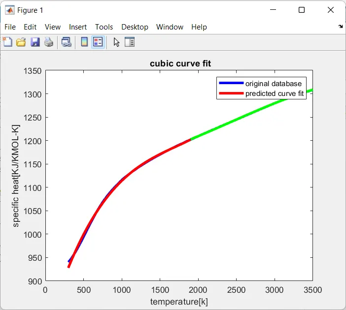

  

• Steps to run programme;
  *START THE PROG WITH CLC,CLOSE ALL,CLEAR ALL
  *LOAD THE DATTASET
  *CURVE FITTING TO BE PERFORMED WITH TWO FUNCTIONS POLYFIT AND POLYVAL
  *CURVE IS COMPARED WITH ORIGINAL AND PREDICTED DATASET

  Curve fitting tool box :

  *it is the alternative to compute the best and perfect fit of given dataset.

  *We need to initiate the x and y values and polynomial degrees which compiles to original dataset and results Rsquare,SSE,adjR^2,RSME..
  
  
  * Best fit:-
  It means the difference between actual and predicted values by the equation.

  * Perfect fit:-
  when the curve is analysised at every point SSE is 0.0 and Rsquaredis 1.00.

  How to get best fit:-
  *Degree of polynomial affects the details
  *The higher the polynomial degree the more closely the polynomial fits the data.the lower the polynomial degree have the effect of smoothing the fit.
  *Experiment the random polynomial data in matlab while using polyfit function.
  *The third degree appropriates the sine curve >note 9th degree fit curve more closely but not appropriated sine curve.

• To improve the cubic fit we can use splitwise method into 4 parts to get best fit:-
• matlab programme
  

  clc
  close all
  clear all
  %loading data
  cp_data=load('data123');

  %first column temperature
  temperature=cp_data(:,1);
  %second column specific heat
  cp=cp_data(:,2);

  
  %split wise method into 4 parts

  temp1=temperature(1:800,1);
  cp1=cp(1:800,1);
  temp2=temperature(801:1600,1);
  cp2=cp(801:1600,1);
  temp3=temperature(1601:2400,1);
  cp3=cp(1601:2400,1);
  temp4=temperature(2401:3200,1);
  cp4=cp(2401:3200,1);

  
  %considering third order cubic polynomial eqn y=ax^3+bx^2+cx+d
  %polyfit used to determine coefficients of a,b
  coefficient1=polyfit(temp1,cp1,3);
  coefficient2=polyfit(temp2,cp2,3);
  coefficient3=polyfit(temp3,cp3,3);
  coefficient4=polyfit(temp4,cp4,3);

  %polyval used to determine the predicted value of cp
  predicted_cp1=polyval(coefficient1,temp1);
  predicted_cp2=polyval(coefficient2,temp2);
  predicted_cp3=polyval(coefficient3,temp3);
  predicted_cp4=polyval(coefficient4,temp4);

  %array of temperature and predicted cp
  predicted_cp=[predicted_cp1,predicted_cp2,predicted_cp3,predicted_cp4];
  temp=[temp1,temp2,temp3,temp4];

  %plotting original dataset and predicted dataset curve

  plot(temperature,cp,'LineWidth',3,'Color','b');
  hold on
  plot(temp,predicted_cp,'LineWidth',3,'Color','k');
  % hold on
  % plot(temp2,predicted_cp2,'LineWidth',3,'Color','k');
  % hold on
  % plot(temp3,predicted_cp3,'LineWidth',3,'Color','k');
  % hold on
  % plot(temp4,predicted_cp4,'LineWidth',3,'Color','k');

  legend('original database','predicted curve fit')
  title('curve fit')
  
  xlabel('temperature[k]')
  ylabel('specific heat[KJ/KMOL-K]')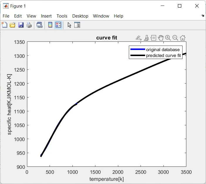

  

• How to make curve fit perfectly?
  *To get a perfect fit,we need to get the value of R_squared equal to 1
  *In curve toolbox set degree to 8 to get best fit of the curve.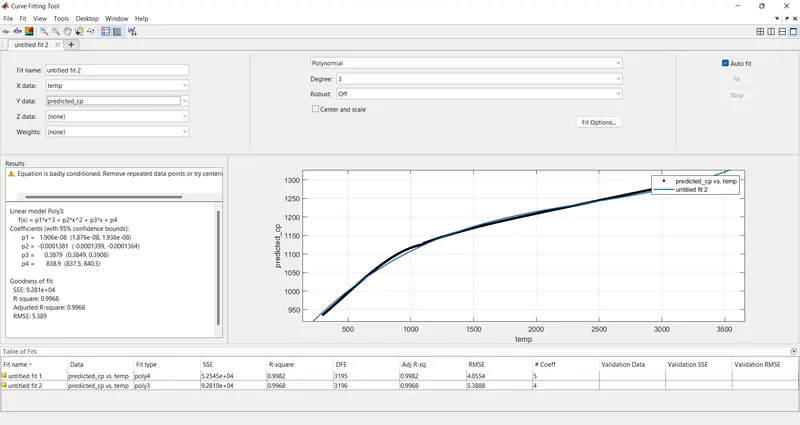
  
• what could be dne to improve the cubic fit?
• When we execute the command we get error saying equation is badly condtioned it can be solved with by'centre the scale option'
  
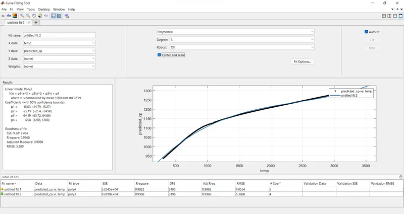
• We can observe the results above the higher the splitting the dataset the better the curve appears:
  
  
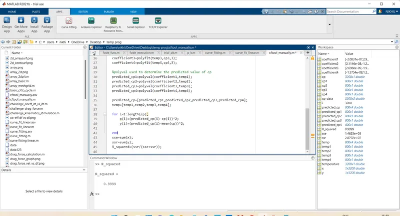
  Curve fitting can be manually calculated by using for loop and compute R_squared
• Matlab Programme
  
  
  conclusion:
• There are many methods to make curve fit properly.
• we need to use higher order of polynomial equation to get best fit.
• Splitting the the data in more parts we get the better output.
• best fit can be achieved by variaying the degree in cf toolbar.
  
  References:-
• How to make curve fit perfectly?
  *To get a perfect fit,we need to get the value of R_squared equal to 1
  *In curve toolbox set degree to 8 to get best fit of the curve.
• https://en.wikipedia.org/wiki/Root-mean-square_deviation
• https://www.mathworks.com/help/curvefit/polynomial-curve-fitting.html