Week 3 - Solving second order ODEs

AIM:-

To simulate the pendulum in MATLAB to solve the second-order equation of the pendulum and to plot the angular displacement and angular velocity.

OBJECTIVE:-

The objective is to write a program that solves the following ODE. This ODE represents the equation of motion of a simple pendulum with damping.

THEORY:-

The ODE represents the equation of motion for the simple pendulum

where,

g = gravity in m/s2,

L = length of the pendulum in m,

m = mass of the ball in kg,

b=damping coefficient.

we have to transform the equation into first-order then we will be able to write in the Matlab code.

We are calling

`theta` =`theta1`

`(d theta)/dt=[d theta1]/dt=theta2----- -(1)`

`(d^2 theta)/dt^2=(d^2 theta1)/dt^2=d/dt((d theta1)/dt)=d/dt (theta2)-----(2)`

`(d^2 theta)/dt^2+b/m*(d theta)/dt+g/l*sin*(theta)=0`

`(d^2 theta1)/dt^2+b/m*(d theta1)/dt+g/l*sin (theta1)`

`(d theta2)/dt+b/m theta2+g/l*sin (theta1)=0`

`(d theta2)/dt = -b/m*theta2-g/l*sin(theta1)`

Now we can put this equation into our Matlab program. And using this equation we will find the angular displacement and angular velocity.

MATLAB FUNCTION PROGRAM:-

function[dtheta_dt] = ode_func(theta,b,g,l,m)

theta1 = theta(1);
theta2 = theta(2);

dtheta1_dt = theta2;

dtheta2_dt = -(b/m)*theta2-(g/l)*sin(theta1);


[dtheta_dt] = [dtheta1_dt;dtheta2_dt];
end

• This is our separate function program which is basically solving the first-order equation which we have generated.
• We have clubbed the value of theta1 and theta2 as theta of 1 and theta of 2 which is basically the theta as it going to show the output in two different columns.
• We are showing our ODE in the form of Matlab code dtheta1_dt = theta2; and the other one isdtheta2_dt = -(b/m)*theta2-(g/l)*sin(theta1);
• With that function, we are making the equation and we are calling this function in our main program.
• This particular function is going to give us results values and time values

MATLAB PROGRAM FOR PENDULUM:-

close all
clear all
clc
 % Simulating program for pendulum 
% initial parameters
b = 0.05;
g = 9.81;
l = 1;
m = 1;

%Initial condition
theta_0 = [0;3];

% time points 
t_span = linspace(0,20,500);

% solve ODE Equation of first order

[t,results] = ode45(@(t,theta) ode_func(theta,b,g,l,m),t_span,theta_0);

%Plotting on graph
plot(t,results(:,l))
hold on
plot(t,results(:,2))
xlabel('Time')
ylabel('angular displacement and angular displacement')
title('Pendulum displacement') 
legend('angular displacement','Angular velocity')
hold off
grid on
% Animation of pendulum

ct = 1;

for i = 1:length(t)
    
    x = sin(results(i,1))*l;
    y = -cos(results(i,1))*l;
    
    figure(2)
    
    plot([-1,1],[0,0],'linewidth',25)
    hold on
    plot([0,x],[0,y],'linewidth',5)
    plot(x,y,'Marker','o','Markersize',25,'Markerfacecolor','g')
    hold off
    axis([-1.5,1.5,-2,2]);
    xlabel('x axis')
    ylabel('y axis')
    title('Pendulum movement')
    
   M(ct) = getframe(gcf);
    ct = ct+1;
end 
% creating movie of pendulum movement

movie(M)
videofile = VideoWriter('pendulum_animation.avi','Uncompressed AVI');
open(videofile)
writeVideo(videofile,M)
close(videofile)

• As the first step will always be to clear all, close all,clc after that we can start writing the code.
• So first we have to define the input parameters as given in the problem. And also the input conditions which has been given are initial angular velocity is 0 and angular displacement is 3 rad/sec.
• We are solving two first-order ODEs one is for angular displacement and the other is for angular velocity.
• We are going to be integrating the ODE system to obtain the solution for which we need to define value for time
• t_span is our time array which goes from 0 to20 seconds with 500 values.
• Then we have to call our ODE function which we already created in another code.
• ode45 is an inbuilt solver in Matlab then we have to put the main inputs as the dependent variable and the independent variable. In our case, theta is our dependent variable and time t is our independent variable so we are saying that our ode is a function of (t, theta) then we are defining our function ode_func(theta,b,g,l,m) this is the calling of our ode function where we have put the input parameters. After that we are providing the initial conditions and after that we provide the integration.
• As we are solving two ODEs this is going to be the column vector we can see in the workspace that the and is in the form of two-column then one column represents the angular displacement and the other column represents the angular velocity.
• We can see the displacement is started with the 0 which is our initial boundary condition and the velocity has started with 3 rad/sec.
• After that we have to plot our angular displacement and velocity for that we used the plot command and plot and label all the essential detailes.
• Then we have made the animation of the pendulum by using all our values time and angular displacement we have made the animation.
• To make this we have used the for loop command and defined the coordinates where the fixed point is supposed to be and we fixed the axis so it will move according to that only.
• x = sin(results(i,1))*l;
  y = -cos(results(i,1))*l; this is what we have to plot on the graph and this is going to give us all the required values where the pendulum is moving with respect to time.
• With respect to our assigned values we have plot the pivot on the co-ordinates [-1,1],[0,0].
• Then we plotted the plunger on[0,x],[0,y] this is going to fixed the point of plunger and will give the animation to it.
• Then by using marker we draw the o shape sphere on the end of the plunger or shaft.
• Then after that we put the movie command to make the movie in the.avi format we open the video file and write the script to the video file and stiched all the images to make the animation and we write the videofile using videowriter command and after putting the M we were able to create the video out of it and then we close the videofile.

RESULTS:-

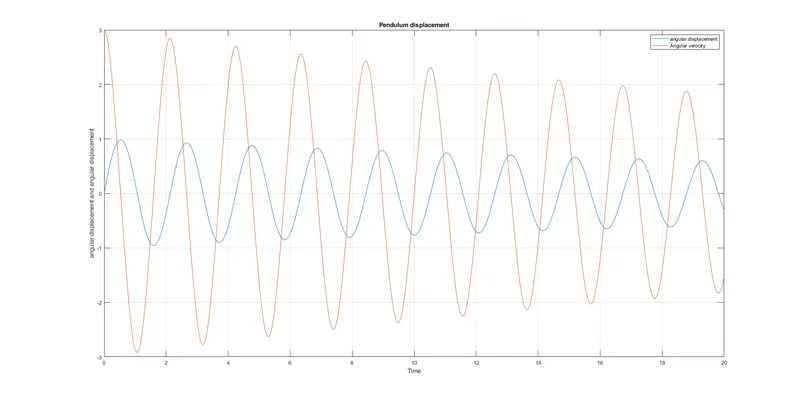
This is our displacement velocity curve with respect to a time where we can see the sinosiadle waveform-like shape of the curve. As the angular displacement is started from the 0 which is the initial condition for it and the angular velocity has started from the initial point 3 rad/sec which is its defined initial condition and with that initial velocity the pendulum was able to move back and forth with respect to its fixed point.

https://youtu.be/ScR5nI3Qmcs by clicking on this link you will be able to see the animation of the pendulum which was made using programming on MATLAB.

CONCLUSION:-

With the help of MATLAB, we solved the second-order ordinary differential equation and also created the animation of the pendulum by using the concept of for loop and also the function program we were able to write the program and performed successfully.