Week 3 - Solving second order ODEs

%function of ode equation

function [dtheta_dt] = ode_int(t,theta,b,g,l,m)

theta1=theta(1);
theta2=theta(2);
dtheta1_dt=theta2;
dtheta2_dt=-(b/m)*dtheta1_dt-(g/l)*sin(theta1);
dtheta_dt=[dtheta1_dt;dtheta2_dt];

end


%program to solve second order differential equations

clear all
close all
clc

%inputs

b=0.05;
g=9.81;
l=1;
m=0.1;

%intial condition

theta_0=[0;3];

%time

t_span=linspace(1,20,500);

%ode equation eith attributes of displacement and velocity

[t,results]=ode45(@(t,theta) ode_int(t,theta,b,g,l,m),t_span,theta_0)

plot(t,results(:,1))
hold on
plot(t,results(:,2))
xlabel('plot')
ylabel('time')

%creating animation

%inputs

x0=0;
y0=0;
l=1;
ct=1;
disp = results(:,1);

for i=1:500

    y1=-l*cos(disp(i));
    x1=l*sin(disp(i));
    figure(2)
   

   

    plot([x0,x1],[y0,y1]) 
    hold on

    plot(x1,y1,"Marker",".",'MarkerSize',40) 
    axis([-2,2,-2,0.5]);

    pause(0.03);
    hold off
    
    M(ct)=getframe(gcf);
    ct=ct+1;
end

% these are the set of commands helps to bind the plots into animation ansd
% stores in the form of a video

movie(M);
videofile=VideoWriter("simplependulum.avi",'Uncompressed AVI');
open(videofile)
writeVideo(videofile,M)
close(videofile)

result:

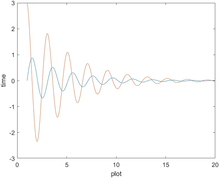
animation:

AIM:

TO PERFORM A PROGRAM IN MATLAB TO SOLVE THE ODE EQUATION WHICH REPRESENTS THE EQUATION OF MOTION OF A SIMPLE PENDULUM WITH DAMPING

GOVERNING EQUATIONS

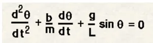
b= damping cofficient

m = mass of bob

g= gravity

L = length of the pendulum

sin@ = angle between mean and extreme positions of pendulum

THE ABOVE EQUATION REPRESENTS EQUATION OF MOTION OF A SIMPLE PENDULUM WITH DAMPING . INTEGREATING THE EQUATION REPRESENTS THE VELOCITY WHILE INTEGRATING TWICE GIVES THE ANGULER DISPLACEMENT

THETA VALUE REPRESENTS THE ANGLE BETWEEN THE PENDULUM AND MEAN POSITION OF THE PENDULUM

THE DISPLACEMENT AND VELOCITY OF SIMPLE PENDULUM AT ANY POINT CAN BE DETERMINED BY THE ANGLE

ODE45:

SYNTAX OF ODE45:

[t,y] = ode(odefun,tspan,yo)

odefun REPRESENTS THE ODE FUNCTION IN WHICH DIFFERENTIAL EQUATION IS SOLVED TO GET VALUES OF VELOCITY AND DISPLACEMENT

tspan is array of values of time

y0 is initial conditions of velocity and displacement

OBJECTIVES:

THE OBJECTIVES OF PROJECT IS TO SOLVE THE ODE EQUATION OF THE SIMPLE PENDULUM EQUATION WITH DAMPING. AFTER SOLVING THE EQUATION PLOT

THE CURVES OF ANGULAR DISPLACEMENT AND VELOCITY IN PLOT AND TIME AS LABELS

AND ALSO TO CREATE A ANIMATION OF THE SIMPLE PENDULUM USING THE IMAGES PLOTTED

BODY:

%Function of the ode equation

function [dtheta_dt] = ode_int(t,theta,b,g,l,m)

theta1=theta(1);
theta2=theta(2);
dtheta1_dt=theta2;
dtheta2_dt=-(b/m)*dtheta1_dt-(g/l)*sin(theta1);
dtheta_dt=[dtheta1_dt;dtheta2_dt];

end

%program to solve second order differential equations

clear all
close all
clc

%inputs
b=0.05;
g=9.81;
l=1;
m=0.1;

%intial condition
theta_0=[0;3];
%time
t_span=linspace(1,20,500);

%ode equation

[t,results]=ode45(@(t,theta)ode_int(t,theta,b,g,l,m),t_span,theta_0)

plot(t,results(:,1))
hold on
plot(t,results(:,2))
xlabel('plot')
ylabel('time')

%creating animation

%inputs
x0=0;
y0=0;
l=1;
ct=1;

for i=1:500

y1=-l*cos(results(i,1));
x1=l*sin(results(i,1));
figure(2)

plot([x0,x1],[y0,y1])
hold on

plot(x1,y1,"Marker",".",'MarkerSize',40)
axis([-2,2,-2,0.5]);

pause(0.03);
hold off

M(ct)=getframe(gcf);
ct=ct+1;
end

% these are the set of commands helps to bind the plots into animation ansd
% stores in the form of a video

movie(M);
videofile=VideoWriter("simplependulum.avi",'Uncompressed AVI');
open(videofile)
writeVideo(videofile,M)
close(videofile)

RESULT:

graph:

animation:

videolink: https://youtu.be/Dqj3L77HSn8

CONCLUSION:

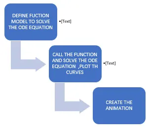
SOLVING TH ODE EQUATION OF THE SIMPLE PENDULUM WITH DAMPING CAN BE DIVIDED IN THREE PARTS FIRST WE HAVE TO DEFINE THE FUNCTION TO SOLVE THE ODE

SECOND STEP TO FOLLOW IS TO SOLVE THE ODE AND PLOT THE ANGULAR DISPLACEMENT AND VELOCITY

AT LAST CREATE THE ANIMATION BY KNOWING THE ABOVE SEQUENCE WE CAN SIMPLY PERFORM THE PROJECT