Week 3 - Solving second order ODEs

AIM: To write a program in MATLAB that solves the following ODE which represents the equation of motion of a simple pendulum with damping.

THEORY:

A pendulum is a weight suspended from a pivot so that it can swing freely. When a pendulum is displaced sideways from its resting, equilibrium position, it is subject to a restoring force due to gravity that will accelerate it back toward the equilibrium position. When released, the restoring force acting on the pendulum's mass causes it to oscillate about the equilibrium position, swinging back and forth.

The motion of the pendulum can be studied using ordinary differential equation. The ODE which represents the equation of motion of a simple pendulum with damping is stated as below.

In the above equation,

g = gravity in m/s^2

L = length of the pendulum in m

m = mass of the ball in kg

b=damping coefficient.

Now we will convert the second order ODE into two first order ODE in order to solve the same.

(d^2theta)/dt^2` + `(b/m) (d theta)/dt` + `(g/L) sintheta` = 0

Let θ = θ1

`(dθ)/dt`= `(dθ1)/dt` = θ2

`(d^2θ1)/dt^2` = `(dθ2)/dt`

Hence `(dθ2)/dt` + `(b/m) θ2` + `(g/L)sinθ1` = 0

`(dθ2)/dt` = - (`(b/m) θ2` + `(g/L)sinθ1`)

PROGRAM:

FUNCTION CODE

function [dtheta_dt] = ode_func(theta,b,g,l,m)
 
theta_1 = theta(1);
theta_2 = theta(2);
dtheta_1_dt = theta_2;
dtheta_2_dt = -(b/m)*theta_2-(g/l)*sin(theta_1);
dtheta_dt = [dtheta_1_dt ; dtheta_2_dt];
end

MATLAB CODE

close all
clc
 
%Inputs
b = 0.05;
g = 9.81;
l=1;
m=1;
theta = [0;4];
tspan = linspace(0,20,300);
ct=1;
[t,results] = ode45(@(t,theta)ode_func(theta,b,g,l,m),tspan,theta);
 
plot (t,results(:,1))
xlabel('Time')
ylabel('Displacement')
hold on
plot (t,results(:,2))
xlabel('Time')
ylabel('Angular velocity')
 
for i=1:length(results(:,1))
    x0 = 0;
    y0 = 0;
    x1 = 1*sin(results(i,1));
    y1 = -1*cos(results(i,1));
    figure(2)
    plot(x0,y0,'.','markers',10)
    hold on
    plot([-0.5,0.5],[0,0]);
    line([x0,x1],[y0,y1]);
    hold on
    plot(x1,y1,'.','markers',20);
    hold off
    grid on
    axis([-1.5 1.5 -1.5 0.5])
    pause(0.001);
    M(ct)=getframe(gcf);
    ct=ct+1;
end
 
movie(M);
videofile = VideoWriter ('ode_function.avi');
open(videofile);
writeVideo(videofile,M);
close(videofile)

EXPLANATION OF THE CODE:

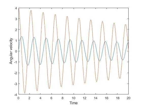
First the inputs has been defined like b,g,l and m. Initial conditions are defined i.e. theta = [0;4]; where initial displacement is 0 and initial angula velocity is 4. Simulation time is defined using linspace command between 0 and 20.

In order to solve the second oredr ODE we need to first convert them to systems of first-order differential equations, and then solve those systems. A function is created in order to solve the same.

Now MATLAB solver ode45 is used to solve the same. Then the results are plotted i.e. displacement vs time & angular velocity vs time. For animation, a base for pendulum is created by fixing a point i.e. x0=0 & y0=0. x1 & y1 is varied according to theta values obtained by solving the ODE.

Finally a movie is created to capture all the frames using movie command.

ERRORS FACED WHILE PROGRAMMING:

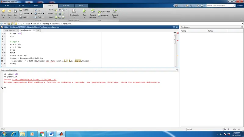
I had made a mistake while defining ODE45 solver which got resolved after after calling it correctly.

OUTPUT GRAPH:

ANIMATION VIDEO:

https://youtu.be/ib455Lkx7BM