Project 2 - Rankine cycle Simulator
AIM:
1) To Develop a basic program that calculates the state points
2) To add the thermodynamic relation to get the points inbetween the state variables.
3) To plot rankine cycle on T-s and H-s curve.
THEORY:
The Rankine cycle is the fundamental operating cycle of all power plants where an operating fluid is continuously evaporated and condensed. The selection of operating fluid depends mainly on the available temperature range.
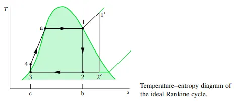
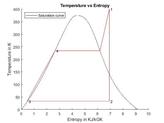
The temperature-entropy (T-s) diagram of this cycle is as shown below. The Rankine cycle operates in the following steps:
- 1-2 Isentropic Expansion. The vapor is expanded in the turbine, thus producing work which may be converted to electricity. In practice, the expansion is limited by the temperature of the cooling medium and by the erosion of the turbine blades by liquid entrainment in the vapor stream as the process moves further into the two-phase region. Exit vapor qualities should be greater than 90%.
- 2-3 Isobaric Heat Rejection. The vapor-liquid mixture leaving the turbine is condensed at low pressure, usually in a surface condenser using cooling water. In well designed and maintained condensers, the pressure of the vapor is well below atmospheric pressure, approaching the saturation pressure of the operating fluid at the cooling water temperature.
- 3-4 Isentropic Compression. The pressure of the condensate is raised in the feed pump. Because of the low specific volume of liquids, the pump work is relatively small and often neglected in thermodynamic calculations.
- 4-1 Isobaric Heat Transfer. High pressure liquid enters the boiler from the feed pump and is heated to the saturation temperature. Further addition of energy causes evaporation of the liquid until it is fully converted to saturated steam.
Work and Heat Transfers
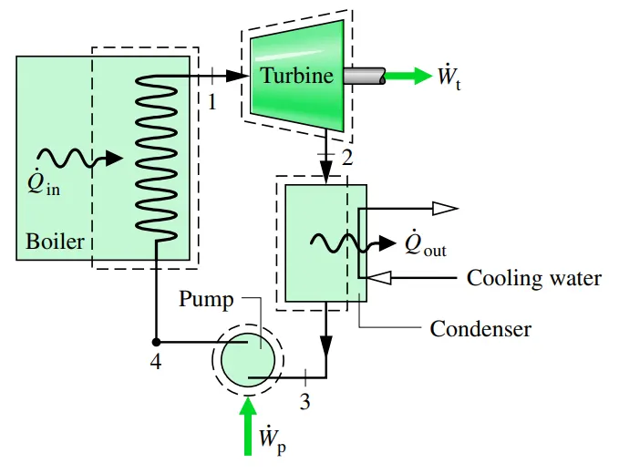
TURBINE: Vapor from the boiler at state 1, having an elevated temperature and pressure, expands through the turbine to produce work and then is discharged to the condenser at state 2 with relatively low pressure. Neglecting heat transfer with the surroundings, the mass and energy rate balances for a control volume around the turbine reduce at steady state to give
W_t = h1-h2
CONDENSER: In the condenser there is heat transfer from the vapor to cooling water flowing in a separate stream. The vapor condenses and the temperature of the cooling water increases. At steady state, mass and energy rate balances for a control volume enclosing the condensing side of the heat exchanger give
Qout = h2-h3
PUMP: The liquid condensate leaving the condenser at 3 is pumped from the condenser into the higher pressure boiler. Taking a control volume around the pump and assuming no heat transfer with the surroundings, mass and energy rate balances give
Wp = h4-h3
BOILER: The working fluid completes a cycle as the liquid leaving the pump at 4, called the boiler feedwater, is heated to saturation and evaporated in the boiler. Taking a control volume enclosing the boiler tubes and drums carrying the feedwater from state 4 to state 1, mass and energy rate balances give
Qin = h1-h4
PERFORMANCE PARAMETERS.
THERMAL EFFICIENCY
The thermal efficiency gauges the extent to which the energy input to the working fluid passing through the boiler is converted to the net work output. Hence the thermal efficiency of the power cycle is
ɳ = (Wt – Wp)/Qin
Back work ratio (BWR):
Another parameter used to describe power plant performance is the back work ratio, or bwr, defined as the ratio of the pump work input to the work developed by the turbine.
bwr = (h4-h3)/(h1-h2) i.e. W_p / W_t
MATLAB CODE:
close all
clc

disp ('Rankine cycle');
disp ('1-2 is isentropic expansion in the turbine');
disp ('2-3 is constant pressure heat rejection by the condensor');
disp ('Isentropic expansion in the pump');
disp ('Constant pressure heat addition to the boiler');

disp ('INPUTS');
P1 = input ('Enter the pressure P1 at the inlet(bar) : ');
T1 = input ('Enter the temperature T1 at the inlet(deg C) : ');
P2 = input ('Enter the pressure P2 at the condenser(bar) :');

%At state 1
h1 = XSteam('h_pT',P1,T1);
s1 = XSteam('s_pT',P1,T1);

%At state 2
s2 = s1;
s2f = XSteam('sL_p',P2);
s2g = XSteam('sV_p',P2);
X2 = (s2-s2f)/(s2g-s2f);
h2f = XSteam('hL_p',P2);
h2g = XSteam('hV_p',P2);
h2fg = h2g-h2f;
h2 = h2f+(X2*h2fg);

%At state 3
P3 = P2;
T3 = XSteam('Tsat_p',P3);
T2 = T3;
h3 = XSteam('hL_p',P3);
s3 = XSteam('sL_p',P3);

%At state 4
s4 = s3;
P4 = P1;
Cp4 = XSteam('Cp_ps',P4,s4);
Cv4 = XSteam('Cv_ps',P4,s4);
k = Cp4/Cv4;
T4 = T3/((P3/P4)^((k-1)/k));
h4 = XSteam('h_ps',P4,s4);

s5 = XSteam('sL_p',P1);
s6 = XSteam('sV_p',P1);
T5 = XSteam('Tsat_p',P1);
h5 = XSteam('hL_p',P1);
h6 = XSteam('hV_p',P1);
T6 = T5;

W_t = h1-h2;
W_p = h4 - h3;
W_net = W_t-W_p;
Q_in = h1-h4;
back_work_ratio = (h4-h3)/(h1-h2);
efficiency = (W_net/Q_in)*100;
SS = 3600/W_net;

%For plotting saturation curve
T = linspace(0,375,1000);
for i=1:length(T)
    sv(i) = XSteam('sV_T',T(i));
    sl(i) = XSteam('sL_T',T(i));
    hv(i) = XSteam('hV_T',T(i));
    hl(i) = XSteam('hL_T',T(i));
end

%Plotting temperature vs entropy graph
figure(1)
hold on
plot(sv,T,'b')
plot(sl,T,'b')
plot ([s1 s2],[T1 T2],'color','r')
plot ([s2 s3],[T2 T3],'color','r')
plot ([s3 s4],[T3 T4],'color','r')
plot ([s4 s5],[T4 T5],'color','r')
plot ([s5 s6],[T5 T6],'color','r')
plot ([s6 s1],[T6 T1],'color','r')
title ('Temperature vs Entropy');
xlabel('Entropy in KJ/kGK');
ylabel('Temperature in K');
legend ('Saturation curve','location','northwest');

text(s1,T1,' 1');
text(s2,T2,' 2');
text(s3,T3,' 3');
text(s5,T5,' 4');

%Plotting enthalpy vs entropy graph
figure(2)
hold on
plot(sv,hv,'b')
plot(sl,hl,'b')
plot([s1 s2], [h1 h2], [s2 s3], [h2 h3], [s3 s4], [h3 h4], [s4 s1], [h4 h1],'color','r')
title ('Enthalpy vs Entropy');
xlabel('Entropy in KJ/kGK');
ylabel('Enthalpy in KJ/kg');
legend ('Saturation curve','location','northwest');

text(s1,h1,'1');
text(s2,h2,'2');
text(s3,h3,'3');
text(s4,h4,'4');

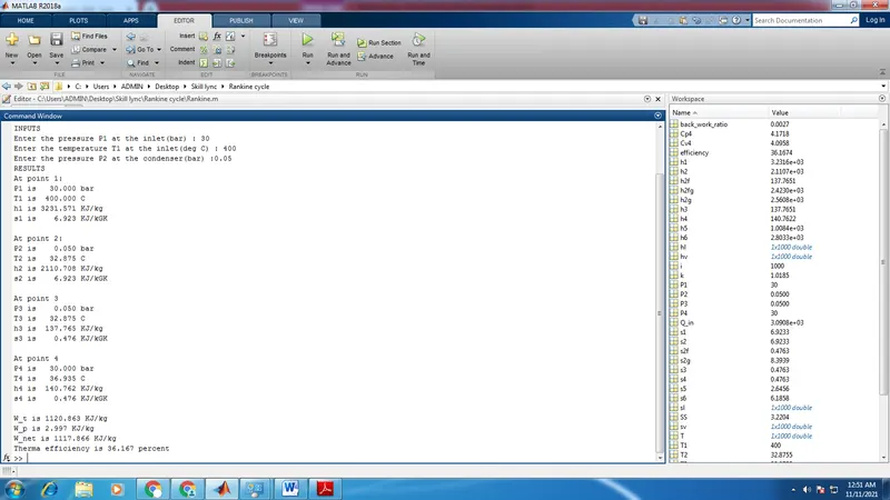
disp('RESULTS');
fprintf('At point 1:\n');
fprintf('P1 is %8.3f bar\n',P1);
fprintf('T1 is %8.3f C\n',T1);
fprintf('h1 is %8.3f KJ/kg\n',h1);
fprintf('s1 is %8.3f KJ/kGK\n\n',s1);
fprintf('At point 2:\n');
fprintf('P2 is %8.3f bar\n',P2);
fprintf('T2 is %8.3f C\n',T2);
fprintf('h2 is %8.3f KJ/kg\n',h2);
fprintf('s2 is %8.3f KJ/kGK\n\n',s2);
fprintf('At point 3\n');
fprintf('P3 is %8.3f bar\n',P3);
fprintf('T3 is %8.3f C\n',T3);
fprintf('h3 is %8.3f KJ/kg\n',h3);
fprintf('s3 is %8.3f KJ/kGK\n\n',s3);
fprintf('At point 4\n');
fprintf('P4 is %8.3f bar\n',P4);
fprintf('T4 is %8.3f C\n',T4);
fprintf('h4 is %8.3f KJ/kg\n',h4);
fprintf('s4 is %8.3f KJ/kGK\n\n',s4);

fprintf('W_t is %.3f KJ/kg\n',W_t);
fprintf('W_p is %.3f KJ/kg\n',W_p);
fprintf('W_net is %.3f KJ/kg\n',W_net);
fprintf('Therma efficiency is %.3f percent\n',efficiency);
EXPLANATION OF THE CODE:
- The input values such as P1, T1 & P2 are given by input command whose values are entered each time when we run the program. Here P1 & T1 is the inlet pressure & temperature of the steam entering the turbine and P2 is the outlet pressure of the steam exiting from the turbine.
- Xsteam data is used to extract the enthalpy, entropy at specific pressure and temperatures for saturated liquid & saturated vapor conditions.
- At state-1, the values of enthalpy and entropy are calculated using below command i.e. h1 = Xsteam (‘h_pT’, P1, T1) which gives enthalpy at pressure P1 & temperature T1.
- At state-2, the dryness fraction is considered for calculation as high pressure steam is converted into low pressure water.
- The variables sf & sg and hf & hg refer to entropy and enthalpy for saturated liquid and saturated gas respectively.
- At State-3, the water is condensed back to its saturation temperature and fed to the pump, hence temperature of water at the exit of the condenser and entry of pump is the same i.e.P3=P2.
- At State-4 i.e. constant pressure heat addition, pressure P4=P1, but the temperature increases on heating at constant Pressure & constant volume as entropy remains same (s4=s3) and hence Cp/Cv=gamma is considered to find temperature T4.
- Now Work done, Heat Evolved, efficiency & SSC are calculated using formulae.
- A temperature range is defined using ‘linspace’ command and for the overall length of this temperature values, enthalpy and entropy of liquid and vapor phases are calculated at every temperature point.
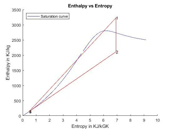
- The saturation curve for liquid phase and vapor phase is plotted by above values of entropy and enthalpy.
- The graph of temperature vs entropy and enthalpy vs entropy is plotted from all the points obtained by the program.
- All the state points are plotted in the same graph using ‘hold on’ command.
- Legend, title and axis label are mentioned for the graphs using appropriate commands.
- Finally the results of the cycle simulation are displayed over command window using ‘fprintf’ command.
ERRORS:
- While ploting the graph of T-s diagram, the sequence of 'x' and 'y' values were not given properly. So the resultant graph was not correct. After typing in the correct sequence the graph was correct and found okay.
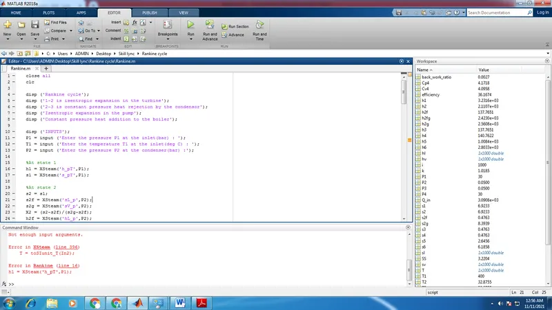
This error was due to not giving sufficient inputs for extracting h1 and s1 data. After giving correct inputs the error got resolved.
RESULTS:
REFERENCES:
https://en.wikipedia.org/wiki/Rankine_cycle
https://energyeducation.ca/encyclopedia/Rankine_cycle
https://thermopedia.com/content/1072