Week 3 - Solving second order ODEs

Simulating a 2nd order ODE system of a simple pendulum :

The above Ordinary Differential Equation is the one which represents the oscillatory motion of the simple pendulum with a bob at the end with a mass of "m", and with the string length of "L", with its damping coefficient "b".

Here, θ is defined as the angular displacement, and the first-order derivative of θ w.r.t to time, i.e.,dθ/dt is defined as the angular velocity and the second derivative of θ w.r.t to time, i.e.,d^2θ/dt^2 is defined as the angular acceleration.

As in manual handwritten terms, the equation containing the higher orders and solving the single independent variable cannot be done by Matlab. Hence we split the higher-order derivatives into first order and the only independent variable containing equations.

BREAKING DOWN OF THE ODE:

Let us assume θ = θ1. Therefore dθ/dt = dθ1/dt = θ2 where, θ2 is the angular velocity.

Now, d^2θ/dt^2 = d^2θ1/dt^2 = dθ2/dt.

Thus, writing the above observations in the ODE of simple pendulum osillation, we'll be getting

dθ2/dt + (b/m)dθ1/dt + (g/L)sinθ1 = 0

Therefore, by taking the 2nd and 3rd term to R.H.S, we get a solution matrix of,

d/dt[ θ1 ; θ2 ] = [θ2 ; -(b/m)θ2-(g/L)sinθ1] wherein (;) represents the column.

We will be using a special type of solver here in Matlab to deal with Ordinary Differential Equations which is called ode45 (we will see that later in the code).

MATLAB CODE:

clear all
close all
clc
%GIVING TIME LIMIT:
%=================
t_0 = linspace(0,20,500)';
%INDICATING INITIAL VALUES OF ANGULAR DISPLACEMENT AND ANGULAR VELOCITY:
theta_0 = [0 3];
%DEFINING THE ODE45 FUNCTION FOR THETA(θ)WITH RESPECT TO THE TIME:
[t,theta] = ode45('Pendulum_challenge',t_0,theta_0);
%PLOTTING THE VARIATION OF ANGULAR VELOCITY W.R.T TO TIME:
figure(1)

plot(t,theta(:,1))
grid on
hold on

%PLOTTING THE VARIATION OF ANGULAR ACCELERATION W.R.T TO TIME:
plot(t,theta(:,2))
xlabel('time')
ylabel('Radians & Omega')
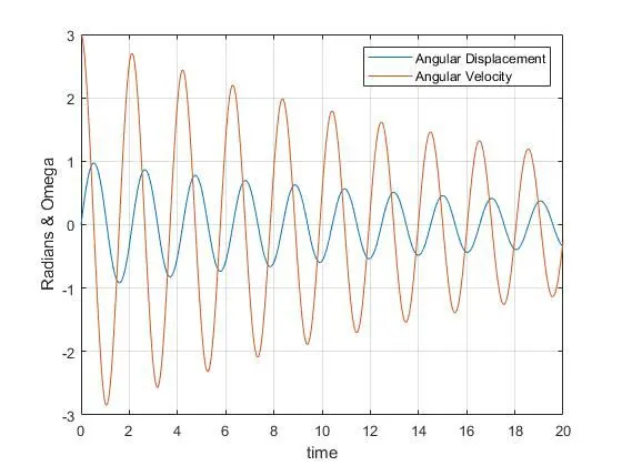
legend('Angular Displacement','Angular Velocity')
%DERIVING THE ANGULAR DISPLACEMENT VALUES IN THE VERY POSSIBLE WAY OF
%GETTING ONLY THROUGH MULTIPLYING TIME DIFFERENCE FOR THE PREFOUND EACH OF
%THE ANGULAR VELOCITY TERMS
%x=theta(:,1);
%for i = 1 : (length(x) -1)
 %expr(i)= x(i) * (t_0(i+1) - t_0(i));
 %%ang_disp = int(expr,[t_0(1) t_0(501)])
%end
%ang_disp = expr';%HERE ARE THE ENTIRE VALUES OF ANGULAR DISPLACEMENT STORED IN (ang_disp)

c=1;
l=1;%LENGTH OF THE STRING:
for i= 1:length(theta(:,1))
    %FIXED END OF THE STRING IS TAKEN TO BE PRESENT AT A COMMON POINT(0,0)
    x_disp_initial = 0;
    y_disp_initial = 0;
    %THE MOVING END WHICH OBVIOUSLY REQUIRES THE ANGULAR DISPLACEMENT IS
    %EQUATED FOR EACH ANG. DISP WHICH WE PRIORLY GOT:
    x_disp_final =-( l * sin(theta(i,1)));
    y_disp_final = -(l * cos(theta(i,1)));
    
    figure(2)%CREATE A FIGURE TO CONTAIN THE ANIMATION
    plot(x_disp_final, y_disp_final, 'o' ,'markersize',20,'markerfacecolor','r')
    hold on
    plot([x_disp_initial x_disp_final],[y_disp_initial y_disp_final],'k','linewidth',2)
    plot([-10.5 10.5],[0 0])
    axis([-1.5 1.5 -2 2])
    xlabel('x-axis');
    ylabel('y-axis');
    title({'Oscillation of Simple Pendulum' , ['Time:', num2str(t_0(i))]})
    
    pause(0.01)%CONTROLS THE PLAYBACK-SPEED OF THE OSCILLATION: 
    hold off
    M(c)=getframe(gcf);%CREATING A MOVIE(M)
    c = c+1;
end
%STITCHING TOGETHER THE IMAGES TO GET AN ANIMATION:
movie(M)
animation= VideoWriter('Simple Pendulum Animation.avi', 'Uncompressed AVI');
open(animation)
writeVideo(animation,M)
close(animation)

FUNCTION:

%CREATE A FUNCTION  
function theta_results = Pendulum_challenge(t,theta_1)
%theta_disp = theta_1(1)';
%GIVE THE INPUT PARAMETERS
b=0.1;%DAMPING COEFFICIENT
g=9.81;%ACC DUE TO GRAVITY
l=1;%LENGTH OF THE STRING
m=1;%MASS OF THE BOB
theta_results = zeros(2,1);%INDICATE THE DEPENDENT VALUE OF THIS FUNCTION A [2X1] ZERO MATRIX
theta_results(1) = theta_1(2);%EQUATE THE 1ST COLUMN OF THE ZERO MATRIX TO ANGULAR VELOCITY 
theta_results(2) = -(b/m)*theta_1(2) - (g/l)*sin(theta_1(1));%EQUATE THE 2ND COLUMN OF THE ZERO MATRIX TO ANGULAR ACCELERATION EQUATION
ang_acc = [-(b/m)*theta_1(2) - (g/l)*sin(theta_1(1))]'
ang_vel = theta_1(2)
end

Here time was taken for 20 seconds with 500 in between seconds for the resulting curve to be better.

Animation of the Simple_Pendulum_Oscillation - Youtube link: https://youtu.be/DyuI6q5WQrE