Week 3 - Solving second order ODEs

Simple Pendulum
Aim:
Solving a second order ordinary differential equation of simple pendulum and showing the effect of damping by an animation.
Objective:
To convert second order ordinary differential equation to 1 order ordinary differential equation.
To create the function using MATLAB in-built function for solving ordinary differential equation.
To plot the displacement and velocity damping through the time stipulated time of simulation.
To make the animation of simple pendulum.

Description:

The differential equation is mostly used to define the complex physics phenomenon in the mathematical way. Differential equation is divided in two different classify as ordinary differential equation and partial differential equation. Solving a 1 order differential is quite easy and require only one constant to define the equation, also it can be also programmed easily. The main effort is taken while solving 2 order differential equation. Most of the fluid equation and some structural phenomenon are defined in the 2 order differential equation which need to solve eventually to simulated the flow or study the structural
behavior.

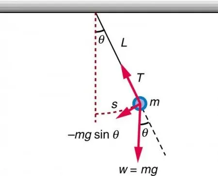
A simple pendulum consists of mass which is attached by the string of length L from a pivot point P. when displaced by initial force the mass gets moved
back and forth performing periodic motion. By applying the Newton’s second law motion we can obtain the equation of motion for simple pendulum.

Code explanation: -
1. The code starts with the inputs which are provided in the problems. Then we make time domain for which the whole code is going to run. It was done by
‘linspace’ command from 0 to 20 seconds with 100 value in between them.
2. After that we provide the initial condition for the angular displacement and velocity which is column vector form, because we need to calculate the both
value from the equation of motion for plotting purpose.
3. The code comprises of function which solves the second order differential equation which is taken inside the main code. The main code has another
function which calculates the array of data for time and displacement.
4. After calculation plotting is done in which subplot command is used, in the first plot first column is plotted and in second subplot second column is plotted
with respect to time.
5. Then we are changing the polar co-ordinate to cartesian co-ordinate because we have used ‘sin’ command instead of ‘sind’ command in function.
6. Then we have created a for loop for which we are creating the frame motion for the simple pendulum and saved in the movie.
The code is given as follows:

close all
clc

b=0.05;
l=1;
m=1;
g=9.81;
theta_0=[0;4];
t_span=linspace(0,20,200);
[t,result]=ode45(@(t,theta) ode_function(b,g,l,m,t,theta),t_span,theta_0);
figure(1)
hold on
plot(t,result(:,1),'color','r');
plot(t,result(:,2),'color','b');
xlabel('Time')
ylabel('Displacemt/Velocity')
legend('Displacement','Velocity')
grid on
ct=1;
for i=1:length(t)
 x0=0;
 y0=0;

 x1=l*sin(result(i,1));
 y1=-l*cos(result(i,1));
 figure(2)
 plot([-2 2],[0 0],'linewidth',3,'color','r');
 line([x0 x1],[y0 y1],'linewidth',4);

 axis([-2 2 -2 2])

 hold on
 plot(x1,y1,'o','markers',20,'markerfacecolor','g');
 hold off

 grid on
 pause(0.03);
 M(ct) = getframe(gcf);
 ct=ct+1;
end
movie(M)
videofile = VideoWriter('Second_order_ODE.avi','uncompressed avi');
open(videofile)
writeVideo(videofile,M)
close(videofile)

The Function is given as:

function [dtheta_dt]=ode_function(b,g,l,m,t,theta)
theta1=theta(1);
theta2=theta(2);
dtheta1_dt=theta2;
dtheta2_dt=-(b/m)*theta2-(g/l)*sin(theta1);
dtheta_dt=[dtheta1_dt;dtheta2_dt];
end

Figure:

https://drive.google.com/file/d/1SOcCAcCWJ3Y_WXY2cZL8NRIi0sor9-16/view?usp=sharing

Animation:

https://youtu.be/zvKDCG3vovc