Week 3 - Solving second order ODEs

Aim: Program that simulates motion of pendulum using 2nd order ODE in MATLAB

Objective:

1) To plot graph of displacement and velocity vs time by solving the given ODE in MATLAB.

2) Creating an animation video of simple pendulum for the given time span.

Code:

Function:

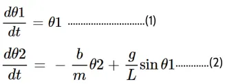
1.The given second order ODE is converted to following 1st order ODE.

function [dtheta_dt] = ode_func(t,theta,b,g,l,m)

    theta1=theta(1);
    theta2=theta(2);
    dtheta1_dt=theta2;
    dtheta2_dt=-(b/m)*theta2-(g/l)*sin(theta1);
    dtheta_dt=[dtheta1_dt;dtheta2_dt];
 end

2. Then, the ODE function is defined seperately for function calling purposes. The "ode_func" contains variables like time (t), theta, damping coefficient (b), length (l), mass (m) as inputs.

3. The values, theta1 and theta2 are defined as solution array followed by definition of ODE's dtheta1_dt and dtheta2_dt.

4. Both the arrays are then combined into the 2D array "dtheta_dt" to form the desired matrix.

5. Later, this function gives the output in the final program which will be a column vector containing two results.

Main Program:

clear all
close all
clc

g = 9.81; % gravity in 'm/s^2'
l = 1 ; % length of the pendulum in 'm'
m = 1; % mass of the ball in 'kg'
b = 0.05; % damping coefficient

%For t=0
theta_0 = [0;3]; %angular displacement= 0;angular velocity=3 m/s
 
t_span = linspace(0,20,500); % 0 to 20 sec time span in equal parts

[t,results] = ode45(@(t,theta)ode_func(t,theta,b,g,l,m),t_span,theta_0); % using ode45 solver

%plotting the graph of time vs displace and velocity
figure(1)
hold on
plot(t,results(:,1),'linewidth',2)
plot(t,results(:,2),'linewidth',2)
title('Simple harmonic motion of pendulum')
xlabel('Time(sec)')
ylabel('Displacement and Velocity')
legend('Angular displacement','angular velocity')
grid on
hold off

%CODE FOR ANIMATION

theta2 = results(:,1);
ct=1;
for i = 1:length(theta2) 
     theta_a = theta2(i);
     
     %intial ang disp of pendulum(x and y)
     x0 = 0; 
     y0 = 0;
     
     %final ang disp of pendulum(x,y)
     x1 = l*sin(theta_a); 
     y1 = -l*cos(theta_a);
     
     %creating animation for the simple pendulum
     figure(2)
     plot([-1 1],[0 0],'color','black','linewidth',3); %for the fixed support
     hold on
     plot([x0 x1],[y0 y1],'color','r','linewidth',2); %for string of the pendulum
     hold on
     plot(x1,y1,'o','markers',20,'markerfacecolor','g') %for the spherical ball
     grid 
     axis([-1.5 1.5 -1.5 1]); %fixing axis
     pause(0.002)
     hold off
     M(ct) = getframe(gcf);
     
     ct = ct+1;
end 

%creating movie and video file 
movie(M)
videofile = VideoWriter('ode_simple_pendulum.avi','uncompressed AVI');
open(videofile)
writeVideo(videofile,M)
close(videofile)

1. Firstly, the given parameters like accelaration due to gravity, damping coefficient, length and mass are intialized .

2. Initial conditions for angular velocity and displacement are set at time t=0.

3. The time span of 0-20 seconds is defined with 500 equally spaced intervals using the linspace command.

4. The ode45 inbuilt solver is used to achieve the output for [t,results] where, (t,theta) are the target constants for which input parameters to ode_func are passed.

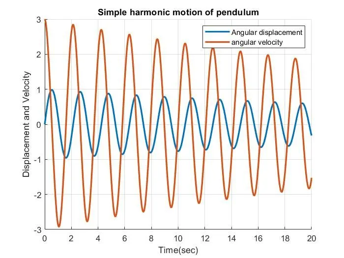
5. Now, two columns containing the values of velocity and displacement is created through which graph can be plotted against time varying from 0-20, representing the graph for motion of simple pendulum.

6. In order to represent the same in the form of animated video, a for loop is created to show the to and fro motion of the simple pendulum. The counter ct will be helpful in capturing the each frame after every loop.

8. Position, dimensions and colors for the simple pendulum are defined. The spherical shape of the the pendulum is achieved through the marker command 'o'. Axis is fixed and pause command is used for the smooth transition of pendulum's motion.

9. A movie is formatted as '.avi' and saved to which the video file is written.

Results:

The following graph has been plotted and animation file is created which can be found in the drive link below.

https://drive.google.com/file/d/1U3CT9Ok6DUOoE1Pg62P3uNNBxf5p_MmB/view?usp=sharing

Conclusion:

It can be observed that the MATLAB is essential is simulating complex models easily and accurately. Also, Maximum no. of oscillations can be damped with an increase in the value of damping coefficient.

Errors faced:

There were no errors faced. Only few warnings due to the use of clear all, and missing semicolons.