Solving second order ODEs

AIM: To write a program in MATLAB to solve a second order ordinary differential equation (ODE) and simulate the pendulum motion.

THEORY:

Ordinary differential equation (ODE):It is a differential equation containing one or more functions of one independent variable and the derivatives of those functions.

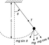
The simple pendulum is a mechanical system that moves in an oscillatory motion. It consists of a point mass ‘m’ suspended by means of light inextensible string of length ‘L’ from a fixed support. The motion occurs in a vertical plane and is driven by a gravitational force ‘g’.

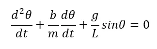
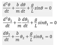
Second order ODE:

-------(1)

g = gravity (m/s²)

L = length of the pendulum (m)

m = mass of the bob (kg)

b = damping coefficient (Ns/m)

Solution:

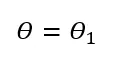
Let’s assume that;

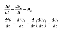
Differentiating with respect to t;

-------(2)

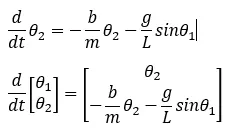
From eq-(1)

Therefore;

PROCEDURE:

Function

function [dtheta_dt]=ode_func(t,theta,b,g,l,m)
theta1=theta(1);
theta2=theta(2);
dtheta1_dt=theta2;
dtheta2_dt=-(b/m)*theta2-(g/l)*sin(theta1);
dtheta_dt=[dtheta1_dt;dtheta2_dt];

end

Explanation

1. The program for function of ode45 is written as per the solution of the second order ODE.
2. This function takes the user input for time, theta, damping coefficient, gravity, length of the pendulum and mass of the bob.

Program

clear all
close all
clc

%Input parameters
%damping coefficient (Ns/m)
b=0.05;

%gravity (m/s^2)
g=9.81;

%length of pendulum (m)
l=1;

%mass of the bob (kg)
m=1;

%Initial conditions
theta_0=[0;3];

%Time points
t_span=linspace(0,20,600);

%ODE
[t,results]=ode45(@(t,theta) ode_func(t,theta,b,g,l,m),t_span,theta_0);

displacement=(results(:,1));
velocity=(results(:,2));

%Plotting the figure
figure(1)
plot(t,displacement)
hold on
plot(t,velocity)
grid on
ylabel('Plot')
xlabel('Time')
title('Plot of angular displacement and angular velocity')
legend('Angular displacement','Angular velocity')

a=1;
for i=1:length(displacement)
    THETA=displacement(i);
    
    %bar
    figure(2)
    plot([-0.5 0.5],[0 0],'linewidth',5,'color','b')
    hold on
    
    %String initial position
    x0=0;
    y0=0;

    %String final position
    x1=l*cos(3*pi/2+THETA);
    y1=l*sin(3*pi/2+THETA);
    
    %String plot
    plot([x0 x1],[y0 y1],'linewidth',2,'color','r')

    %bob
    plot(x1,y1,'O','markersize',25,'markerfacecolor','y','markeredgecolor','y')
    axis([-2 2 -2 2])
    grid on
    hold off
    
    M(a)=getframe(gcf);
    a=a+1;
    
end

movie(M)
videofile=VideoWriter('Pendulum.avi');
open(videofile)
writeVideo(videofile,M)
close(videofile)

Explanation

1. We begin with clear all, close all, clc to get rid of any previous data, plots, etc.
2. We then define all the input parameters required for our program such as damping coefficient, gravity, length of the pendulum and mass of the bob.
3. We then define the angular displacement, angular velocity which in this case is 0 and 3 when t=0. Also, the time duration during which the pendulum oscillates is defined as t_span=20 seconds in this case.
4. Then the ode45 command is called to solve the second order ODE as mentioned earlier.
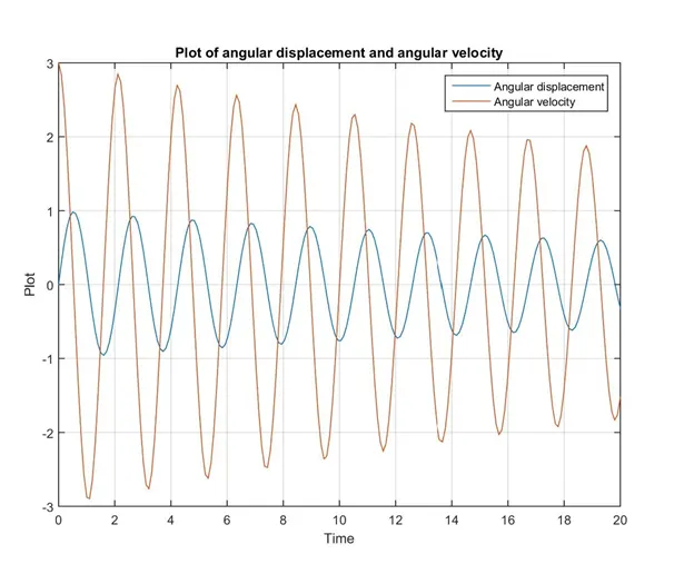
5. Using hold on command angular displacement v/s time and angular velocity v/s time is plotted in a single plot. The X-axis is labelled as ‘Time’ using xlabel command and the Y-axis is labelled as ‘Plot’ using ylabel The plot is given the title of ‘Plot of angular displacement and angular velocity’ using title command. Also, a legend is created representing angular displacement in blue and angular velocity in red using the legend command.
6. For the pendulum animation, for loop is used so that for every value of angular displacement the position of the bob changes according to the angular displacement.
7. The plot command is used to create a visual of the pendulum. In this plot, the bob and one end of the string change their positions according to angular displacement. Whereas, one end of the string remains fixed at the origin. Also, the axis command is used to define the visible area of the plot.
8. All the plots are saved in M at one time using a after which the loop starts again.
9. The movie command is used to create a movie and saved in .avi format.

RESULTS:

Plot:

Link for pendulum animation: click here