Week 3 - Solving second order ODEs

AIM:

i)To write a program which solves the second order ordinary differential equation of pendulum using Matlab or Octave.

ii)To simulate the motion of pendulum with respective parameters and creating an animation.

DAMPING CO-EFFECIENT:

I'd like to share here what damping coeffecient is and how it's value affects the system performance before proceeding to the code.

A damping coefficient is a material property that indicates whether a material will bounce back or return energy

Such measures are required when evaluating material and system responses to dynamic loading conditions
Materials with high damping coefficients are used in applications of shock absorption, vibration control
For example, a basketball has a low damping coefficient (a good bounce back).
If the bounce is caused by an unwanted vibration or shock, a high damping coefficient in the material will diminish the response.
It will swallow the energy and reduce the undesired reaction.

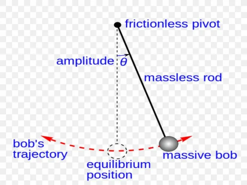
PENDULUM IMAGE:

This image shows the movement of pendulum that we are going to write the code for.

CODE SCRIPTED IN OCTAVE:

MAIN PROGRAM:

clear all
close all
clc

%defining inputs(given value)

b = 0.05; %damping coeffecient_c

L = 1; %length of arm m

m = 1; % mass of the sphere kg

g = 9.81; %acceleration due to gravity m/s^2

%definig initial condition

theta_0 = [0;3];

%defining duration of oscillation

osci_time = linspace(0,20,100);


%calling function and solvind second order ODE

[t,solution]=ode45(@(t,theta) second_ode(t,theta,b,g,m,L),osci_time,theta_0);

%plotting 
%uses subplot to put together all curves in one figure

subplot(2,3,1)

plot(t,solution(:,1)) %(:,1) seperates the two plot as 1 and 2

hold on

plot(t,solution(:,2),'color','r')
title('time vs ang_velocity/ang_displace')
xlabel('Time')
ylabel('Ang_velocity/ang_displace ')

hold off

subplot(2,3,2)
plot(solution(:,1),solution(:,2))
xlabel('displacement,rad')
ylabel('angular velocity,rad/s')


ct=1;
for i = 1:length(t)
  
  x0 = 0;
  y0 = 0;
  
  
  x1= L.*sind(solution(i,1));
  y1= -L.*cosd(solution(i,1));
  
  x3=-1;
  x4=1;
  
 
  
  subplot(2,2,3)
   
  plot([x0 x1],[y0 y1],'linewidth',2,'color','g')%plotting fixed point
  
   line([x3 x4],[y0 y0],'linewidth',3,'color','k') %plotting the support beam
   
   hold on
   
   plot( x0, y0,'marker','o','markersize',10,'markerfacecolor','r')
  
  hold on
  
   %plot for the bob in pendulum
  
  plot( x1, y1,'marker','o','markersize',20,'markerfacecolor','r')
  
  hold off
  
  axis([-2 2 -2 2])
  
 
  
  pause(0.3)
  
  
  %command for creating animation
  t=sprintf('secondODE%d.png',ct);
  saveas(gca,t)
  
  ct=ct+1;
  
end

#Here i use octave for programing the code.

EXPLANATION OF THE CODE:

1.Program starts with the clearing command.

2.The inputs required for the code such as damping co-effecien,length,bob mass,g is given as per the value provided.

3.The initial condition for the dispalcement and angular velocity is given.The oscillatiion time is given using the linspace command.

4.function is used to define the reduction of second order differential equation ,here two theta values are created and it is used for breaking the equation which is given in the code.The second order differential equation which we reduced is

`(d^2theta)/dt^2+b/m*(d theta)/dt+g/L*sintheta`

5.The equation is reduced using the ODE45 inbuilt command in matlab/octave.(ODE-ordinary differential equation).

6.After reducing we get three results one for time,second for andular displacement third for,angular velocity we get value from 0 to 20 which is the range we give in time.

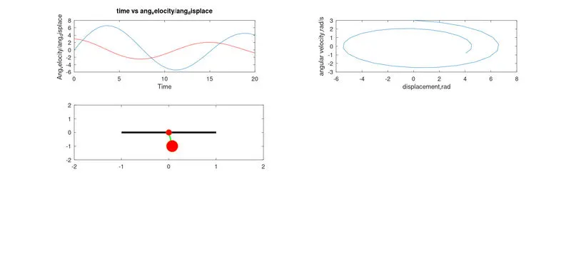
7.Then we get to start plot with different values which is attached in the below image.

8.Inorder to create animation we use for loop for recursive operation till the length if t ,the length command is used for the number of values in the array.

9.Inside the for loop we define the coordinates for the pendulum arm and the bob.since the pendulum oscillates for an angle from the middle axis.

10.The bob is created using the marker command which gives a sphere structure in the respectiive coordinates.

FUNCTION PROGRAM:

function [v] = second_ode(t,theta,b,g,L,m)
  %assigning theta 1and 2
  theta1 = theta(1);
  theta2 = theta(2);
  dtheta1_dt = theta2;
  dtheta2_dt = -(b/m)*theta2-(g/L)*sind(theta1);
  v = [dtheta1_dt;dtheta2_dt];
end

ERRORS:

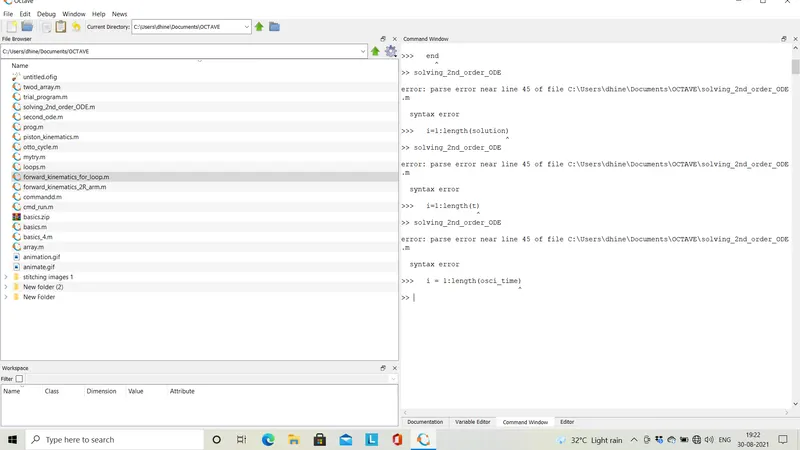
Here i use two end command in the for loop so it shows a syntax error.

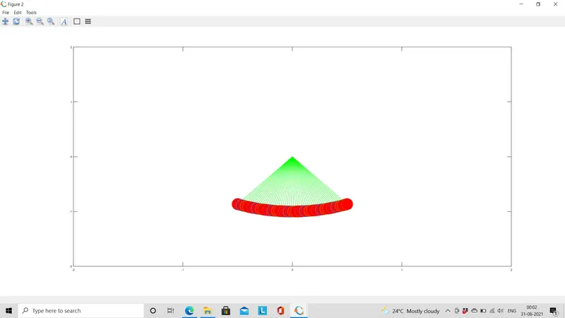
When the axis command is written above the plot command.

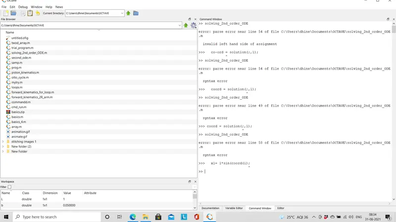
syntax for assigning variable is given wrongly.

PLOT FIGURES:

i) The first plot describes time vs ang_velocity/ang_displace,blue line depicts the time vs dispacement and another one is for time vs angular_velocity.

ii)The second plot is for displacement vs angular velocity.

iii)The third plot is for pendulum bob simulation which is written in the for loop

CONCLUSION:

The animation for the swing of pendulum is created using the sprintf command where we get every image of the respective position of pendulum seperately.

The created image is saved seperately ussing the saveas(gca) command.Then by using command prompt we will stitch the images with magick *.png output.gif command .

The videofile for the animation of pendulum bob is attached here.