Week 3 - Pitot tube
Pitot static tube:
The pitot static tube consists of two concentric tubes. The central tube with open end pointing upstream of the fluid flow and the other closed at the end but with small holes drilled at right angles to the direction of the flow. The central tube pressure is equal to the static pressure and the dynamic pressure, wheras the outer tube pressure is the static pressure only.
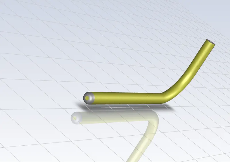
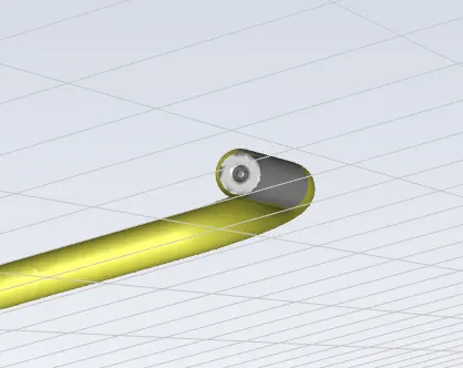
Basically, a pitot tube is used in wind tunnel experiments and on airplanes to measure flow speed. It's a slender tube that has two holes on it. The front hole is placed in the airstream to measure what's called the stagnation pressure. The side hole measures the static pressure. By measuring the difference between these pressures, you get the dynamic pressure, which can be used to calculate airspeed.
On an airplane, the pitot tube can be mounted in a number of ways, including jutting out from the edge of the wing or sticking up from the fuselage.
- The tubes recording static pressure and the stagnation pressure are usually combined into one instrument known as Pitot static tube
Fig 16.4 Pitot Static Tube
- The tube for sensing the static pressure is known as static tube which surrounds the pitot tube that measures the stagnation pressure.
- Two or more holes are drilled radially through the outer wall of the static tube into annular space. The position of these static holes is important. Downstream of the nose N, the flow is accelerated somewhat with consequent reduction in static pressure. But in front of the supporting stem, there is a reduction in velocity and increase in pressure.
- The static holes should therefore be at the position where the two opposing effects are counterbalanced and the reading corresponds to the undisturbed static pressure. Finally the flow velocity is given by
`v= ((2*delP)/rho)^0.5`
`delP=P_T-P_S`
`P_T`is total pressure and`P_s`is the static pressure
This can be obtained using the Bernoulis equation:
`P_1/(rho_1)+(v_1^2/(2*g))=P_0/(rho_0)+V_0^2/(2*g)`
Since the the fluid is brought to rest at the nose, the stagnation velocity is zero. The stagnation pressure is the total pressure. Rearranging the above equation, the velocity of the flow can be obtained.
In aircraft, the static pressure is generally measured using the static ports on the side of the fuselage. The dynamic pressure measured can be used to determine the indicated airspeeds of the aircraft. The diaphragm arrangement described above is typically contained within the airspeed indiocator which converts the dynamic pressure to an airspeed reading by means of mechanical levers.
The fluid coinsiderd is incompressible
CFD analysis:
- The meshed file is imported into ansys fluent
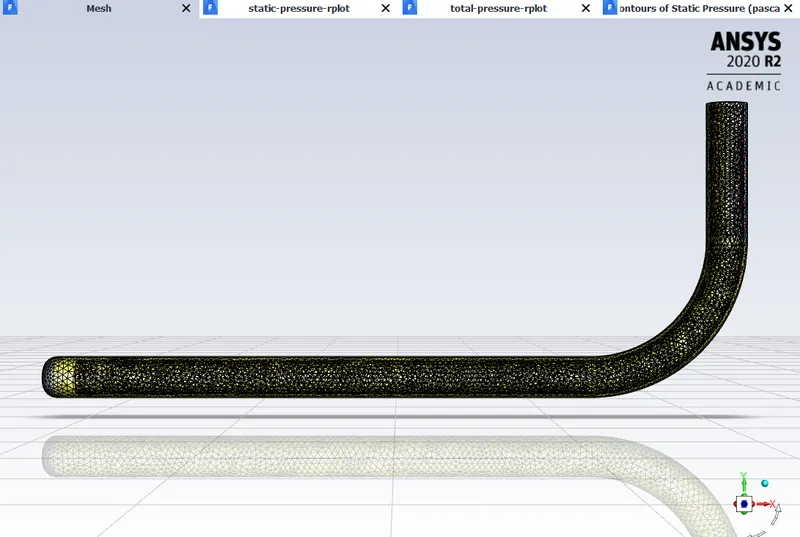
- Mesh check and quality check is performed:
| minimum orthogonal quality | 1.60126e-01 |
| maximum aspect ratio | 1.95073e+01 |
- Under the physics tab, the operating conditions is openned. The operating pressure is set to 0. This is done, since we are dealing with absolutre pressure here.
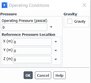
- Since temperature is not a point of concern here, the energy is not turned on.
- To model the viscous model:
`Re=(rho*V*D)/(mu)`
Here, D is the characteristic length.
Since Reynolds number is below 2000, the flow is considered laminar.
- density of air is taken as 0.86 kg/m^3 , `P=rho*R*T` this formulation is used.
- For Boundary conditions:
1) Inlet = Velocity inlet
Three cases are considered here ;
- V= 100 m/s and pressure 33287 Pa
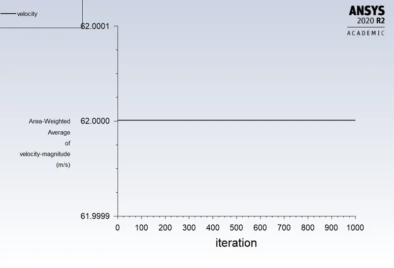
- V=62 m/s and pressure 67580 Pa
- V= 240 m/s and pressure -2817 Pa
2) Outlet = pressure outlet
- Gauge pressure at the outlet is same as the pressure provided at the inlet.
3) All walls are no slip walls
- Solver = Pressure based solver
The pressure-based solver employs an algorithm which belongs to a general class of methods called the projection method . In the projection method, wherein the constraint of mass conservation (continuity) of the velocity field is achieved by solving a pressure (or pressure correction) equation. The pressure equation is derived from the continuity and the momentum equations in such a way that the velocity field, corrected by the pressure, satisfies the continuity. Since the governing equations are nonlinear and coupled to one another the solution process involves iterations wherein the entire set of governing equations is solved repeatedly until the solution converges.
Two pressure-based solver algorithms are available in ANSYS FLUENT. A segregated algorithm, and a coupled algorithm.
The pressure-based coupled algorithm solves a coupled system of equations comprising the momentum equations and the pressure-based continuity equation. in the coupled algorithm, a single step in which the coupled system of equations are solved. The remaining equations are solved in a decoupled fashion .
Since the momentum and continuity equations are solved in a closely coupled manner, the rate of solution convergence significantly improves when compared to the segregated algorithm. However, the memory requirement increases by 1.5 - 2 times that of the segregated algorithm since the discrete system of all momentum and pressure-based continuity equations needs to be stored in the memory when solving for the velocity and pressure fields .
- Steady state simulation and velocity formulation is absolute
Solution methods:
Explicit formulation is done.
Pressure based velocity coupling,
Scheme: Coupled
Spatial discretization:
gradient = Least square based
Pressure = Second order
Momentum = Second order upwind
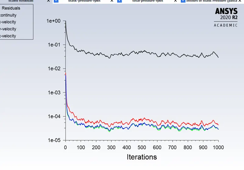
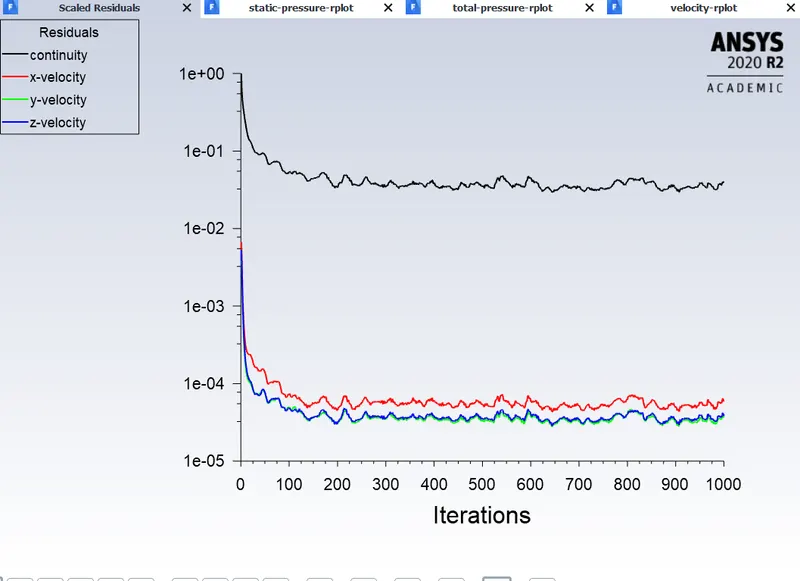
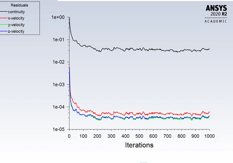
- The convergence criterion for x velocity, y velocity , z velociy and the continiuty equation is set to 0.001
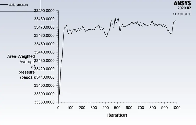
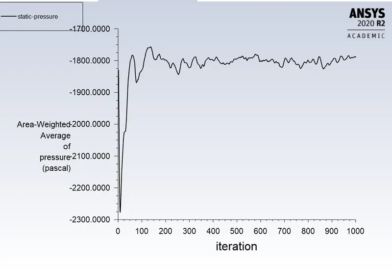
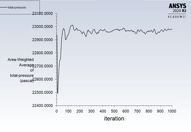
- Under the definitions, three plots are defined, static pressure and total pressure at the inlet and velocity at the inlet.
Hybrid initialization is performed
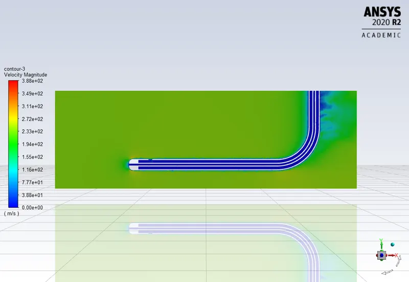
Contours of velocity and static pressure is created at a plane created along the xy plane.
The cases are run foe 1000 iterations .
Results:
- CAse 1:
Velocity = 100 m/s
Pressure = 33287 Pa
1) Residuals plot :
2) static pressure at the inlet plot:
3) Total pressure at the inlet plot:
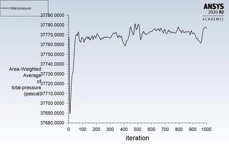

Putting these values in the velocity formula:
`V= ((2*P_T-P_S)/(rho))^0.5`
V= 99.98 m/s
- Case 2:
velocity = 240 m/s
pressure = -2817 Pa
- residuals plot:
- Static pressure at inlet plot:
- Total pressure at inlet:
- Velocity at inlet:
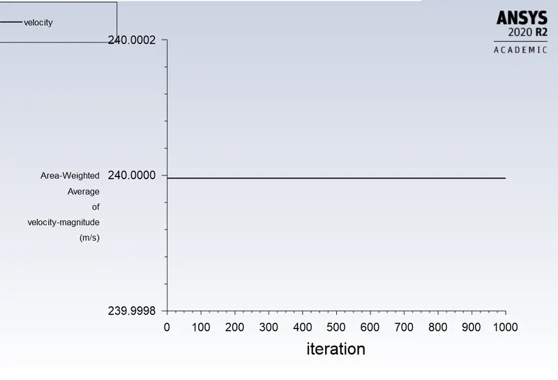

Analytically, V=239.91 m/s
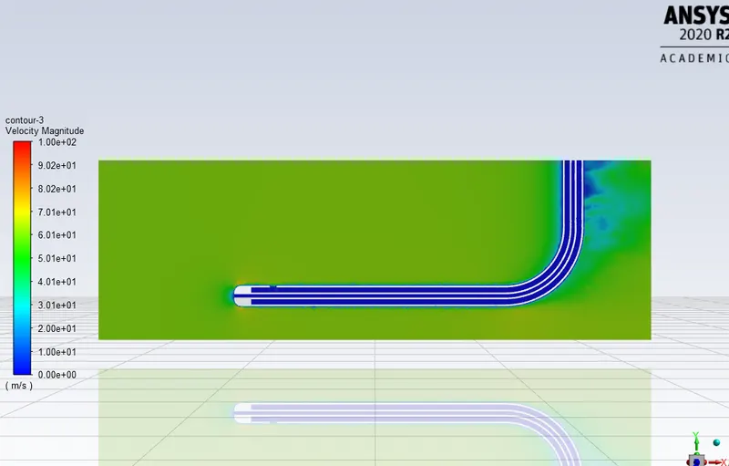
Velocity contour:
Case 3:
- Residual plots:
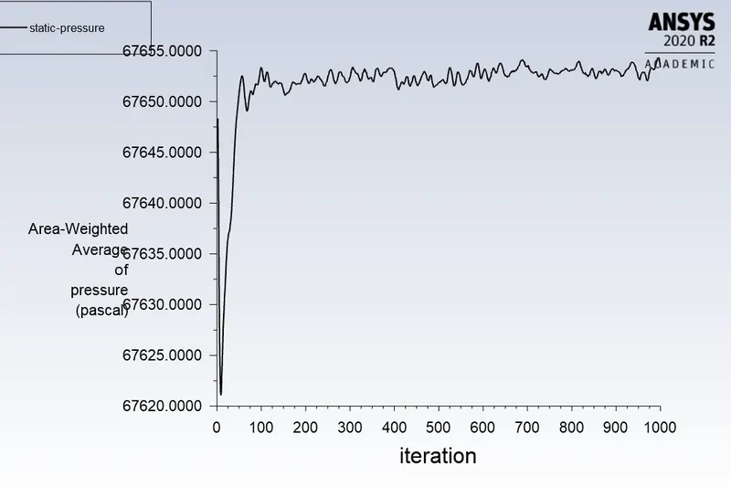
- Static pressure plot:
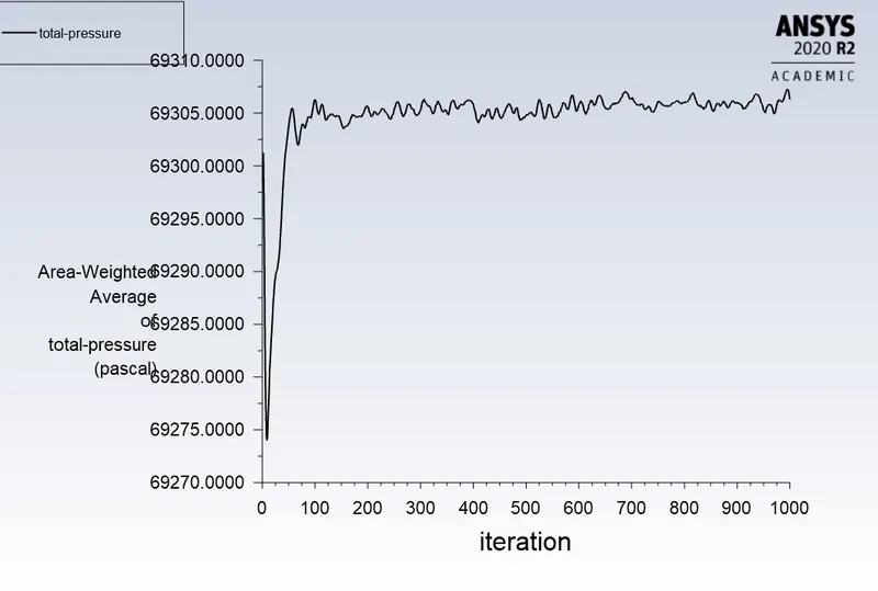
- Total pressure plot:
- Velocity plot:

The analytical equation , and putting these values in it, we get V = 66.85 m/s
`v=(2*(P_T-P_s)/(rho))^0.5`
Velocity contour:
- Comparison:
| Provided data (m/s) | Simulation (m/s) | Percentage error |
| 62 | 66.85 | 7.82 % |
| 100 | 99.98 | 0.02 % |
| 240 | 239.91 | 0.03 % |
- Conclusin:
A literature review of Pitot static tube is performed
Simulation of the pitot static tube for three different cases are performed.