Week 3 - Pitot tube
- Aim:
- Explain about pitot-static tube and also establish a relationship between Total (stagnation) pressure and static pressure.
- Perform a steady state simulation to calculate the Velocity change along the domain and find the percentage from the given data.
- Post process and plot the necessary contours and justify the results.
- Theory:
1. Pitot-static tube:
A pitot tube, also known as pitot probe, is a flow measurement device used to measure fluid flow velocity. The pitot tube was invented by the French engineer Henri Pitot in the early 18th century and was modified to its modern form in the mid-19th century by French scientist Henry Darcy. It is widely used to determine the airspeed of an aircraft, water speed of a boat, and to measure liquid, air and gas flow velocities in certain industrial applications.
The basic pitot tube consists of a tube pointing directly into the fluid flow. As this tube contains fluid, a pressure can be measured; the moving fluid is brought to rest (stagnates) as there is no outlet to allow flow to continue. This pressure is the stagnation pressure of the fluid, also known as the total pressure or (particularly in aviation) the pitot pressure.
The measured stagnation pressure cannot itself be used to determine the fluid flow velocity (airspeed in aviation). However, Bernoulli's equation states:
- Stagnation pressure = static pressure + dynamic pressure
Which can also be written

Solving that for flow velocity gives

where
- u is the flow velocity;
- `P_t` is the stagnation or total pressure;
- `P_s` is the static pressure;
- and `rho` is the fluid density.
NOTE: The above equation applies only to fluids that can be treated as incompressible. Liquids are treated as incompressible under almost all conditions. Gases under certain conditions can be approximated as incompressible.
The dynamic pressure, then, is the difference between the stagnation pressure and the static pressure. The dynamic pressure is then determined using a diaphragm inside an enclosed container. If the air on one side of the diaphragm is at the static pressure, and the other at the stagnation pressure, then the deflection of the diaphragm is proportional to the dynamic pressure.
In aircraft, the static pressure is generally measured using the static ports on the side of the fuselage. The dynamic pressure measured can be used to determine the indicated airspeed of the aircraft. The diaphragm arrangement described above is typically contained within the airspeed indicator, which converts the dynamic pressure to an airspeed reading by means of mechanical levers.
Instead of separate pitot and static ports, a pitot-static tube (also called a Prandtl tube) may be employed, which has a second tube coaxial with the pitot tube with holes on the sides, outside the direct airflow, to measure the static pressure.
If a liquid column manometer is used to measure the pressure difference,
 ,
,

where
- `Delta h` is the height difference of the columns;
- `rhol` is the density of the liquid in the manometer;
- g is the standard acceleration due to gravity.
Therefore,

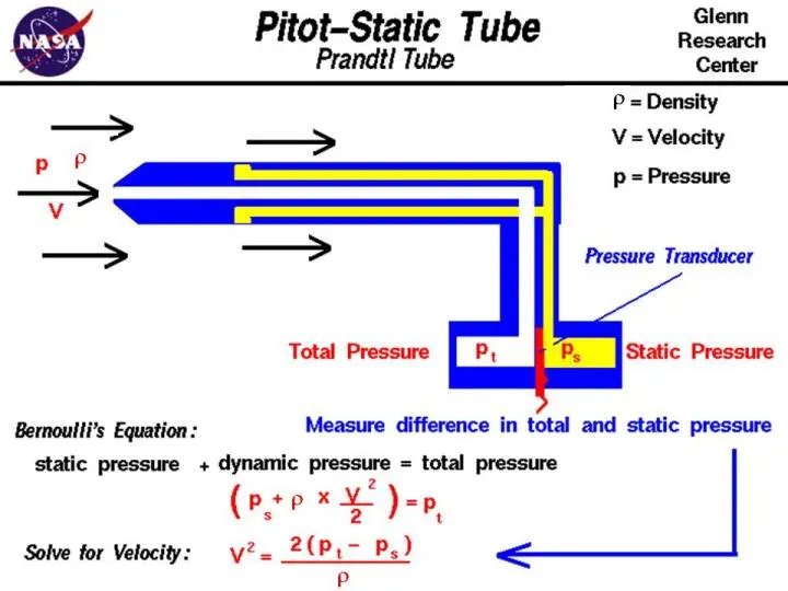
- Relationship between static and dynamic pressure:
Since the outside holes are perpendicular to the direction of flow, these tubes are pressurized by the local random component of the air velocity. The pressure in these tubes is the static pressure (ps) discussed in Bernoulli's equation. The center tube, however, is pointed in the direction of travel and is pressurized by both the random and the ordered air velocity. The pressure in this tube is the total pressure (pt) discussed in Bernoulli's equation. The pressure transducer measures the difference in total and static pressure which is the dynamic pressure q.
measurement = q = pt - ps
- Simulation and results:
- case setup:
Steady-state, pressure based, absolute velocity formulation
Inlet BC:
Velocity= 240, 100, 62
Pressure(gauge)= 2817, 33287, 65780
Outlet:
gauge Pressure= 0
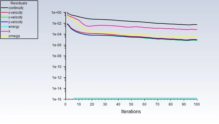
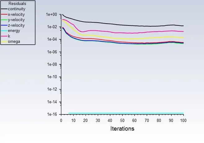
no of cycles= 100
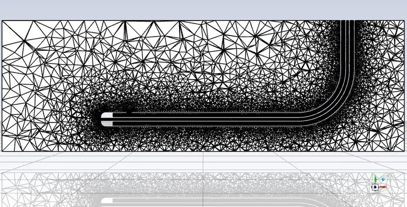
- Mesh:
- Post-processing (Plots and contours)
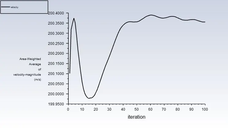
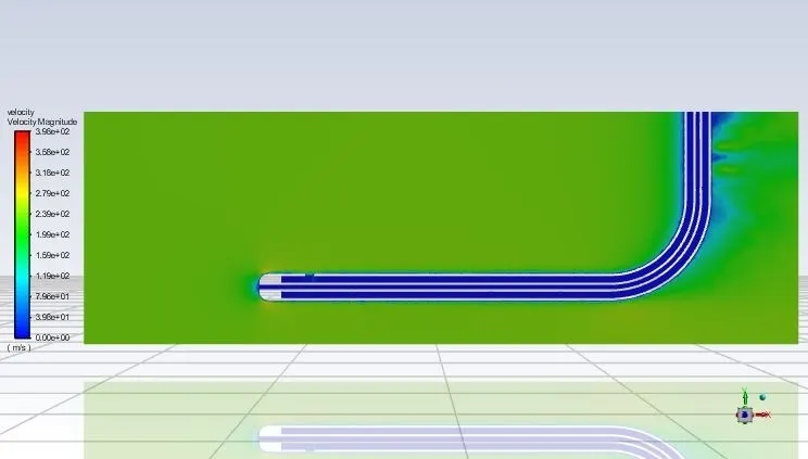
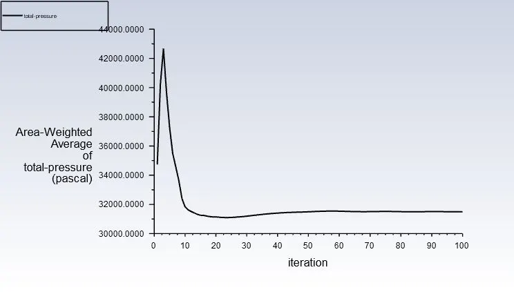
a. Velocity at 240m/s and gauge pressure at 2817Pa:
- Residuals:
- Velocity :
- Static pressure:
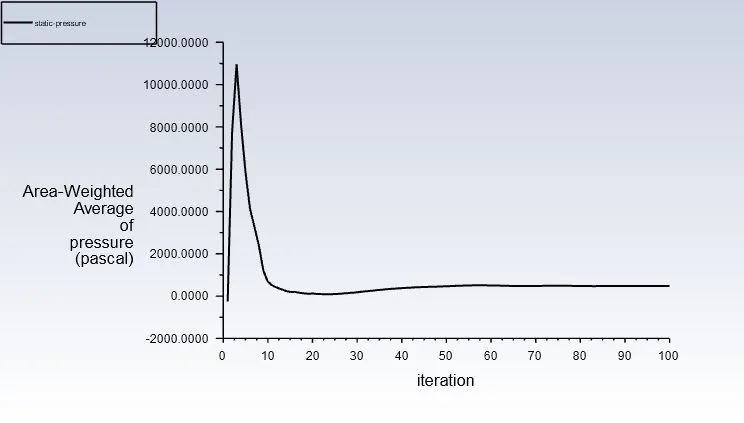
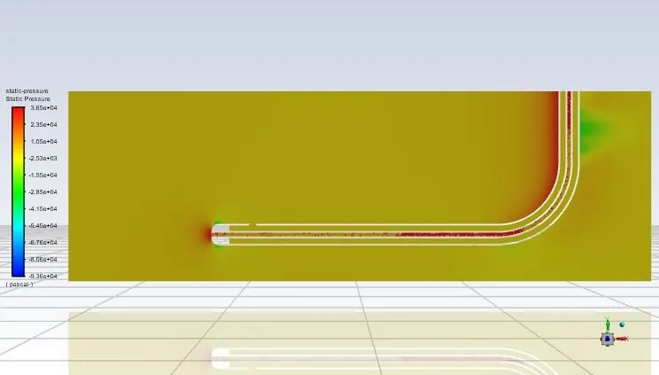
- Total pressure:
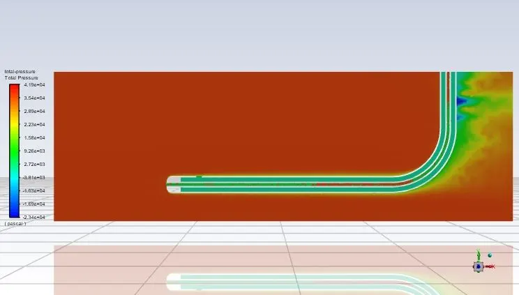
b. Velocity at 100m/s and gauge pressure at 33287Pa:
- Residuals:
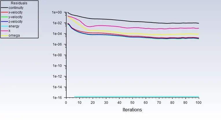
- Velocity:
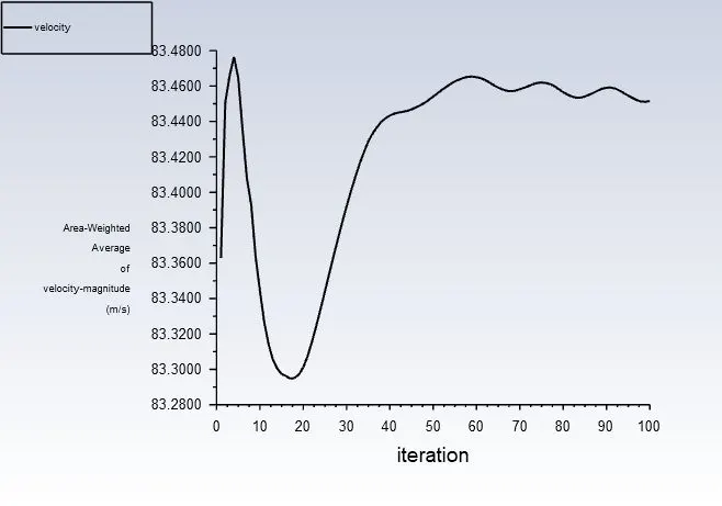
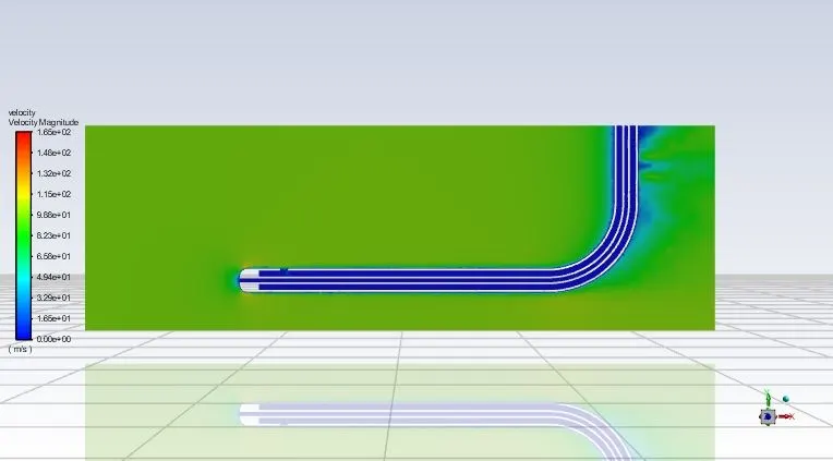
- Static pressure:
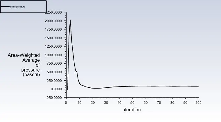
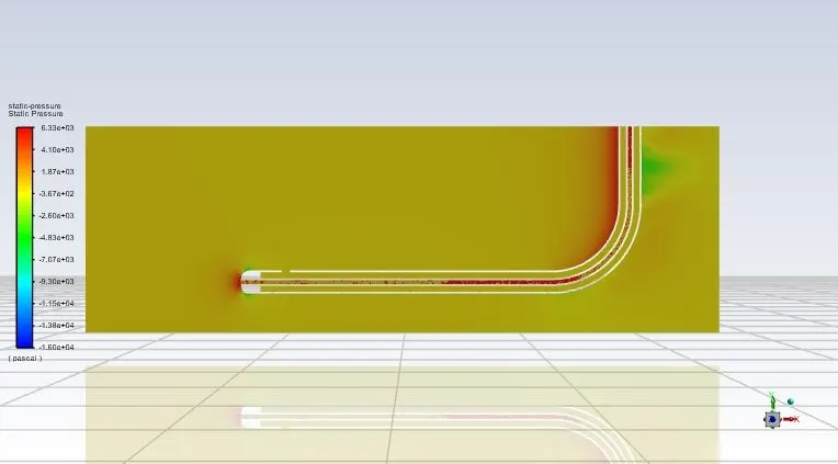
- Total pressure:
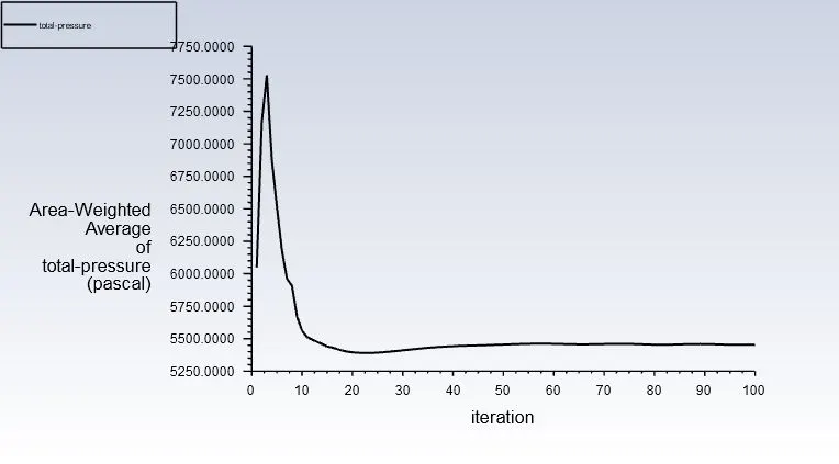
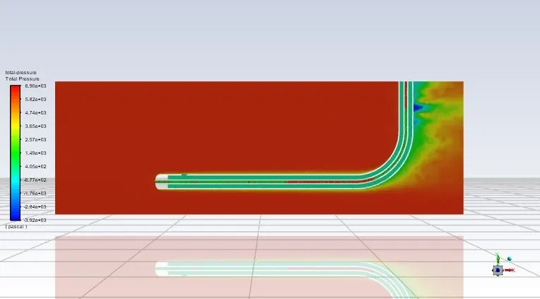
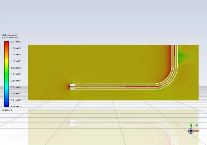
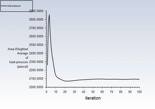
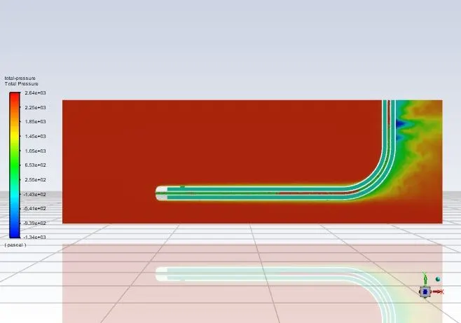
c. Velocity at 62m/s and gauge pressure at 65780Pa:
- Residuals:
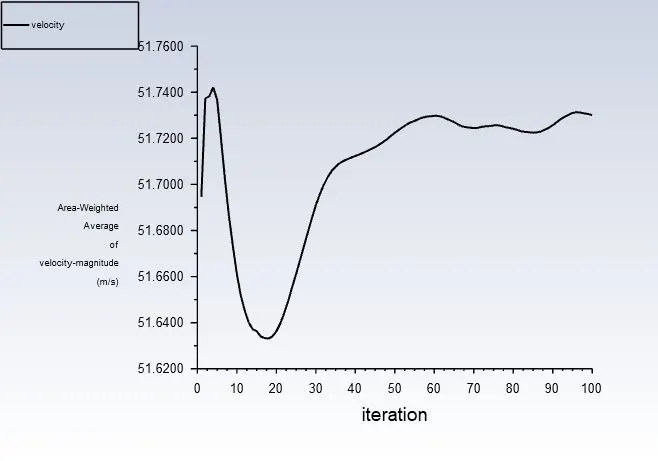
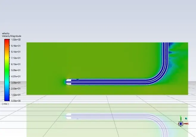
- Velocity:
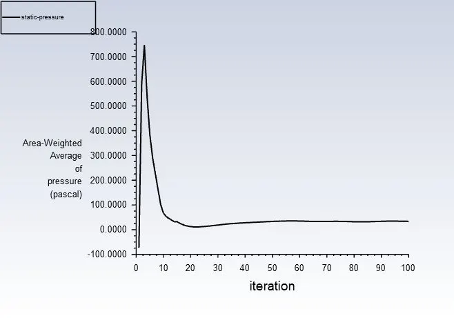
- Static pressure:
- Total pressure:
- Results and Conclusion:
After calculating the Velocities by usng the formula, we get:
| Velocity m/s (Given) | Gauge Pressure Pa (Given) | Static pressure Pa | Total pressure Pa | Velocity m/s | Error percentage (%) Velocity |
| 240 | 2817 | 478.26 | 31500.44 | 225.05 | 6.22 |
| 100 | 33287 | 84.461 | 5454.99 | 93.63 | 6.37 |
| 62 | 65780 | 33.57 | 2093.99 | 57.99 ~ 58 | 6.45 |
The comparison of the actual and analytical results of velocity is performed by calculating the error and the error is around 5% which is acceptable for this kind of simulation.