Week 3 - Pitot tube

1(a). Pitot and Pitot-Static Probes:

Pitot probes (also called pitot tubes) and pitot-static probes, named after the French engineer Henri de Pitot (1695-1771), are widely used for flow speed measurement.

A pitot tube is just a tube with a pressure tap at the stagnation point that measures stagnation pressure, while a pitot-static probe has both a stagnation pressure tap and several circumferential static pressure taps and it measures both stagnation and static pressures.

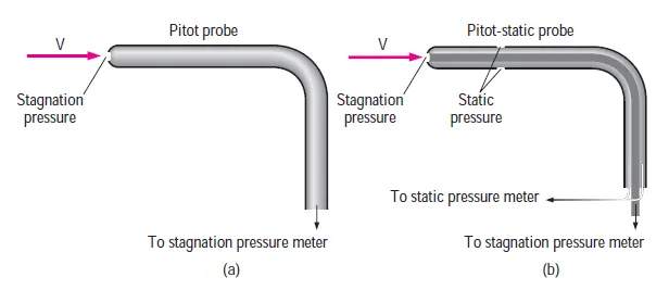
Figure: (a) A pitot tube measure the stagnation pressure at the nose of the probe (b) a pitot-static tube measures both stagnation pressure and static pressure

Pitot was the first person to measure velocity with the upstream pointed tube, while French engineer Henery Darcy (1803-1858) developed most of the features of the instruments we use today, including the use of small openings and placement of the static tube of the same assembly. Therefore, it is more appropriate to call the pitot-static probes Pitot-Darcy probes.

The Pitot static probe measures local velocity by measuring the pressure difference in conjunction with Bernoulli's equation. it consists of a slender double tube aligned with the flow and connected to a differential pressure meter. the inner tube is fully open to flow at the nose and thus it measures the stagnation pressure at that location (point 1). the outer tube is sealed at the nose, but it has holes on the side of the outer wall (point 2) and thus it measures the static pressure.

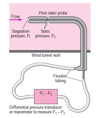
Applybernoullis equation,

`P_1/(rhog)+V_1^2/(2g)+z_1=P_2/(rhog)+V_2^2/(2g)+z_2`

`z_1approxz_2` and `V_1=0` because of stagnation condition

`V_2=V=sqrt((2(P_1-P_2))/rho)`

`V=sqrt((2(stagnation pressure-static pressure))/rho)`

`V=sqrt((2(Dynamic pressure))/rho)`

Note 1: The difference between static and stagnation pressure (which is the dynamic pressure) is directly proportional to fluid density and the square of flow velocity.

Note 2: Pitot static probe should be properly aligned with the flow to avoid significant errors that may be caused by misalignment.

Note 3: it is used to measure the velocity of both liquids and gases. Noting that gases have low densities, the flow velocity should be sufficiently high to develop measurable dynamic pressure.

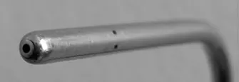
Figure: Close-up of a pitot-static probe, showing the stagnation pressure hole and two of the five static circumferential pressure holes.

1(b)

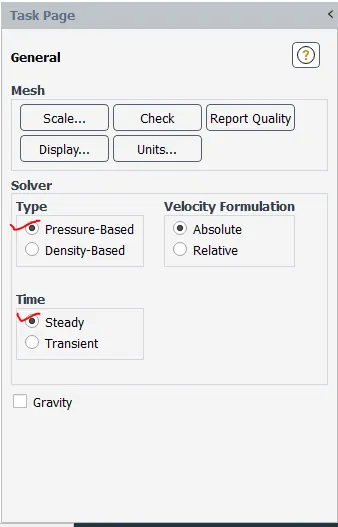
Figure: Solver selection

What is Pressure-based solver and density-based solver:

The pressure-based and density-based approaches differ in the way that the continuity, momentum, and (where appropriate) energy and species equations are solved.

Historically speaking, the pressure-based approach was developed for low-speed incompressible flows, while the density-based approach was mainly used for high-speed compressible flows. However, recently both methods have been extended and reformulated to solve and operate for a wide range of flow conditions beyond their traditional or original intent.

In both methods, the velocity field is obtained from the momentum equations. In the density-based approach, the continuity equation is used to obtain the density field while the pressure field is determined from the equation of state.

On the other hand, in the pressure-based approach, the pressure field is extracted by solving a pressure or pressure correction equation which is obtained by manipulating continuity and momentum equations.

Using either method, Ansys Fluent will solve the governing integral equations for the conservation of mass and momentum, and (when appropriate) for energy and other scalars such as turbulence and chemical species. In both cases a control-volume-based technique is used that consists of:

• Division of the domain into discrete control volumes using a computational grid.

• Integration of the governing equations on the individual control volumes to construct algebraic equations for the discrete dependent variables ("unknowns") such as velocities, pressure, temperature, and conserved scalars.

• Linearization of the discretized equations and solution of the resulting linear equation system to yield updated values of the dependent variables.

Two algorithms also exist under the pressure-based solver in Ansys Fluent: a segregated algorithm and a coupled algorithm. In the segregated algorithm, the governing equations are solved sequentially, segregated from one another, while in the coupled algorithm the momentum equations and the pressure-based continuity equation are solved in a coupled manner.

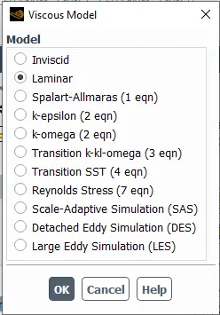
Case 1: V=240 m/s, Gauge Pressure= - 2817 Pa

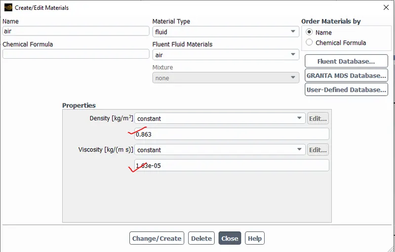
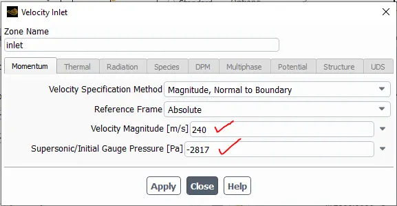
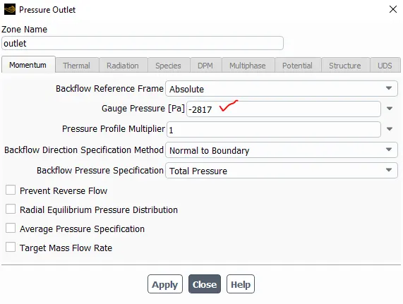
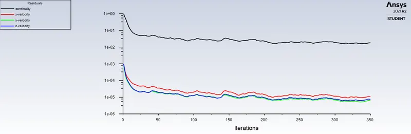
Figure 1(a): Residuals

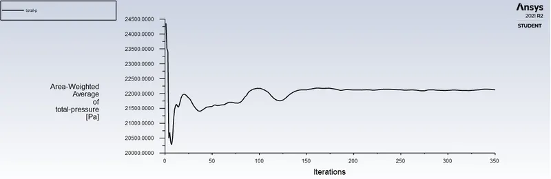
Figure 1(b): Total pressure

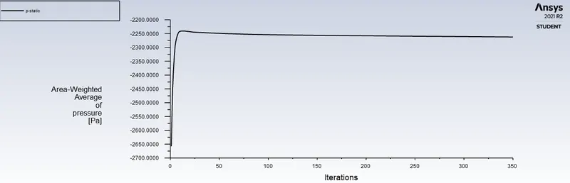
Figure 1(c): Static Pressure

Dynamic pressure =Total pressure - Static pressure

Dynamic Pressure = 22127.264-(-2262.4144)=24,389.6784 Pa

`V=sqrt((2(Dynamic pressure))/rho)`

`V=sqrt((2(24,389.6784))/0.863)`

V=237.745 m/s

Case 2: V=100 m/s, Gauge Pressure= 33287 Pa

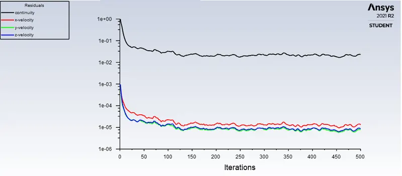
Figure 2(a): Residuals

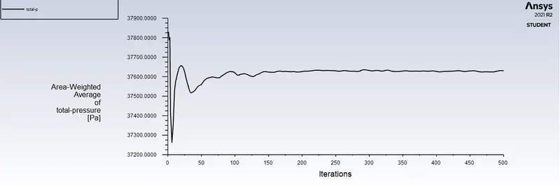
Figure 2(b): Total pressure

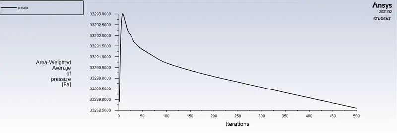
Figure 2(c): Static Pressure

Dynamic pressure =Total pressure - Static pressure

Dynamic Pressure = 37630.729 -33288.593=4,342.136 Pa

`V=sqrt((2(Dynamic pressure))/rho`

`V=sqrt((2(4,342.136))/0.863)=100.313 m/s`

Case 3: V=62 m/s, Gauge Pressure= 65870 Pa

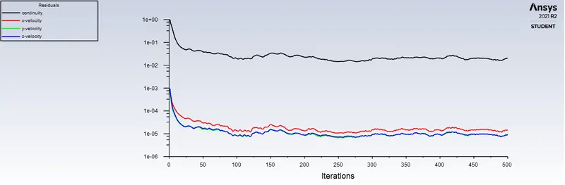
Figure 3(a): Residuals

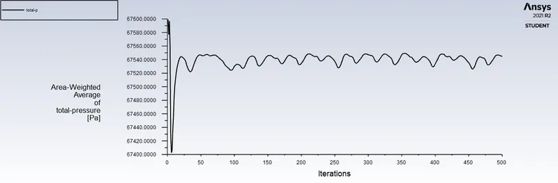
Figure3(b): Total pressure

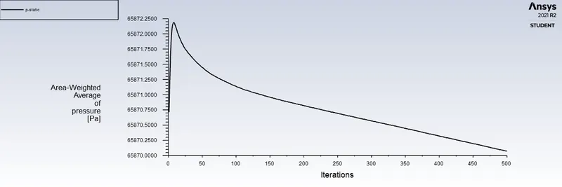
Figure 3(c): Static Pressure

Dynamic pressure =Total pressure - Static pressure

Dynamic pressure = 67544.552 - 65870.067 = 1,674.485 Pa

`V=sqrt((2(Dynamic pressure))/rho`

`V=sqrt((2(1,674.485))/0.863)=62.294 m/s`

S.No.	Gauge Pressure (Pa)	Velocity (m/s)		Error (%)
		Analytical value	Numerical value
1.	-2817	240	237.745	0.939
2.	33287	100	100.313	0.313
3.	65780	62	62.294	0.294