Week 3: Flow over a backward facing step
Assignment Name: Simulate the flow over backward facing step
Objective:
- Run 3 simulations
- 3 different base mesh sizes are,
dx = 2e-3m, dy = 2e-3m, dz = 2e-3m
dx = 1.5e-3m, dy = 1.5e-3m, dz = 1.5e-3m
dx = 1.0e-3m, dy = 1.0e-3m, dz = 1.0e-3m
Introduction
Backward-Facing Step (BFS) flow is one representative model for separation flows, which can be widely seen in aerodynamic flows (aerofoil, spoiler, high attack angle process), engine flows, condensers, vehicles (cars, boat), heat transfer systems, and even the flow around buildings, etc. The flow separation after a simple stage will introduce separation bubble formation, evolution and re-attachment process, which is dependent on the BFS geometric design, the inlet and outlet conditions, turbulent intensity, as well as heat transfer conditions. In the past decades, it has been widely studied by various theoretical, experimental and numerical methods. Considering the importance of BFS flow in both theoretical and engineering aspects, this paper is focused on a review study of BFS flows from fundamental understandings to various experimental and numerical developments in a historical viewpoint. Basic models and the parameter-based after-step flow laws are summarized and categorized in this study. It is shown that the step size (duct expansion ratio) will define the basic re-circulation and re-attachment process, while the coupled effects of inflow parameters and the perturbation designs also help shape the flow behaviors after BFS
Geometry:
1.created geometry of Backward facing step
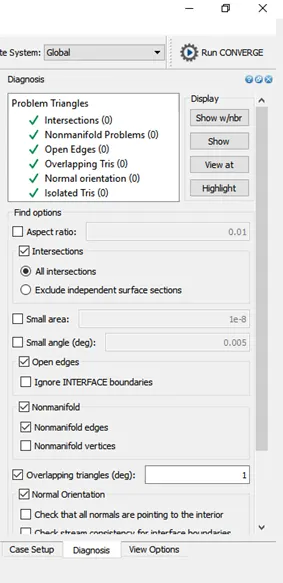
2.checking the normal
3.checking the diagnosis in order to checks error
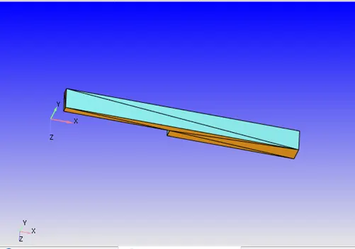
Before proceeding the error in geometry for that
View tab-diagnosis dock-default setting-select the find
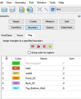
Click on boundary and Create boundary
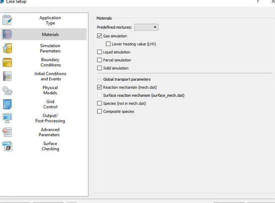
Case Setup
Application Type = Time-based
Materials -
Predefined mixtures = Air
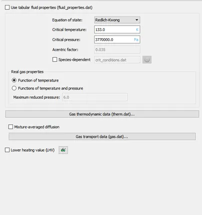
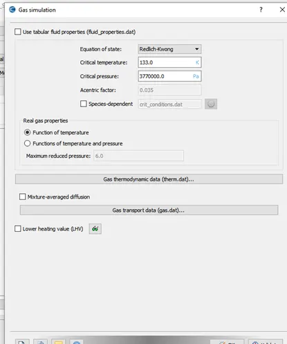
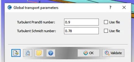
Simulation Parameters-
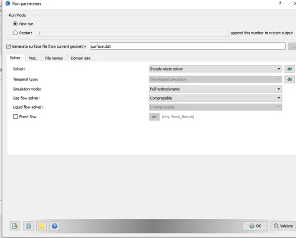
In Run Parameters two main things to be considered: -
select the following solver settings.
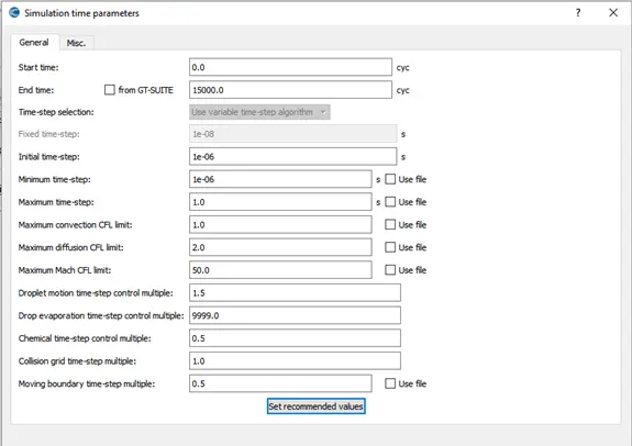
Simulation Time Parameters: -
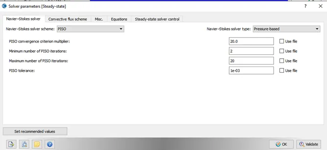
Solver Parameters [Steady-State]-
Navier-Strokes Solver type- pressure based
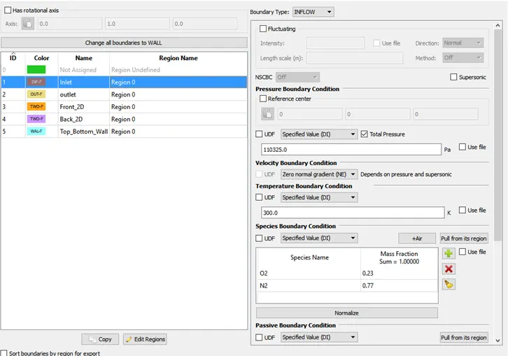
Boundary Conditions-
Inlet
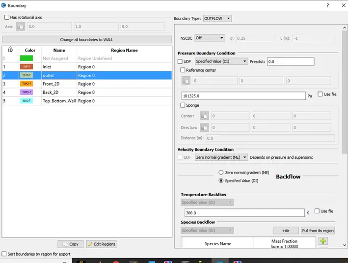
Outlet
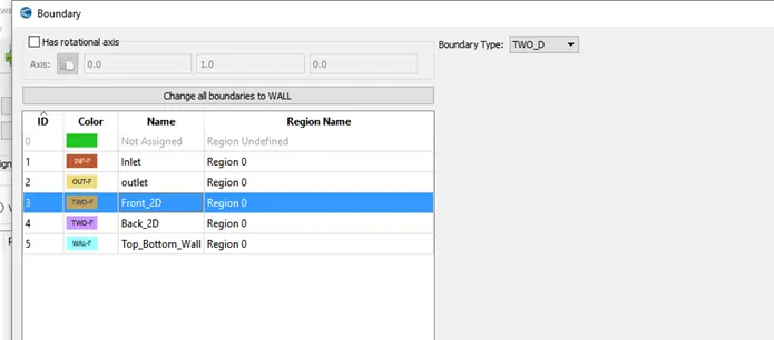
Front 2D
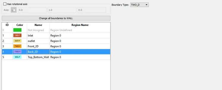
Back 2D
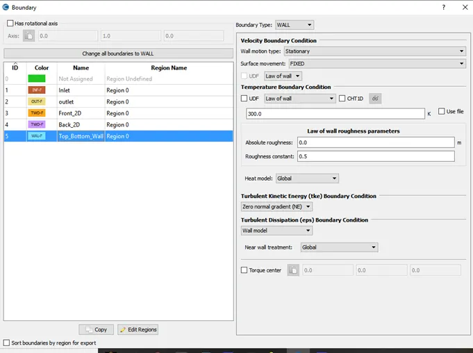
Top_Bottom_wall
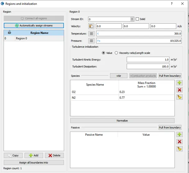
Region and initialization:
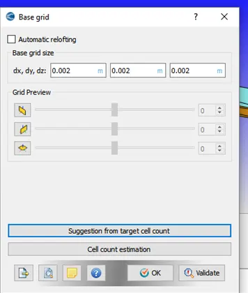
Base grid
Case 1: dx = 2e-3m, dy = 2e-3m, dz = 2e-3m
Case 2 : dx = 1.5e-3m, dy = 1.5e-3m, dz = 1.5e-3m
Case 3 : dx = 1.0e-3m, dy = 1.0e-3m, dz = 1.0e-3m
Note: change base grid size according to your setup
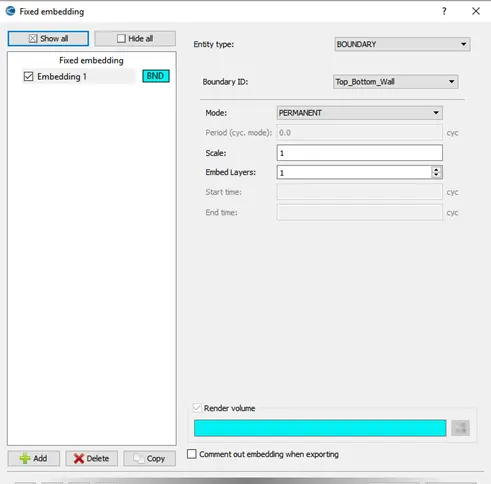
Fixed embedding
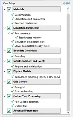
Note: check green tick mark on each option in case setup
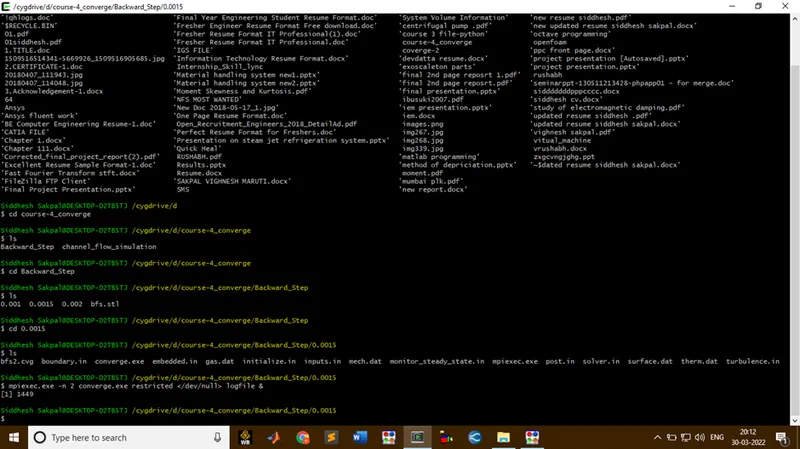
Cygwin Window
Results
Case 1: dx = 2e-3m, dy = 2e-3m, dz = 2e-3m
Mesh
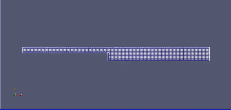
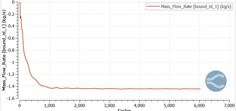
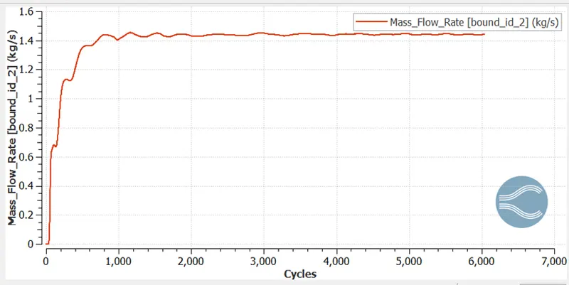
Mass flow rate
Inlet
Outlet
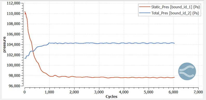
Pressure plot
Inlet And Outlet
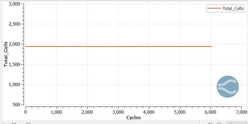
Total cells
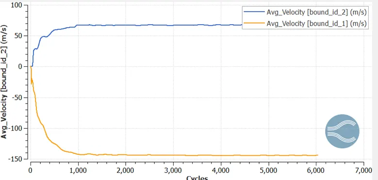
Velocity plot
Inlet And Outlet
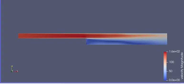
Velocity contour
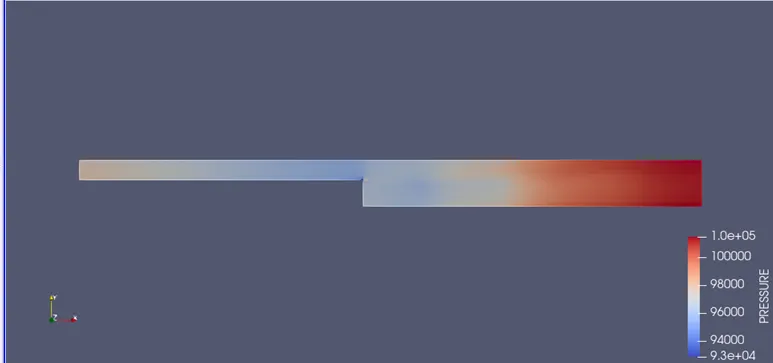
Pressure contour
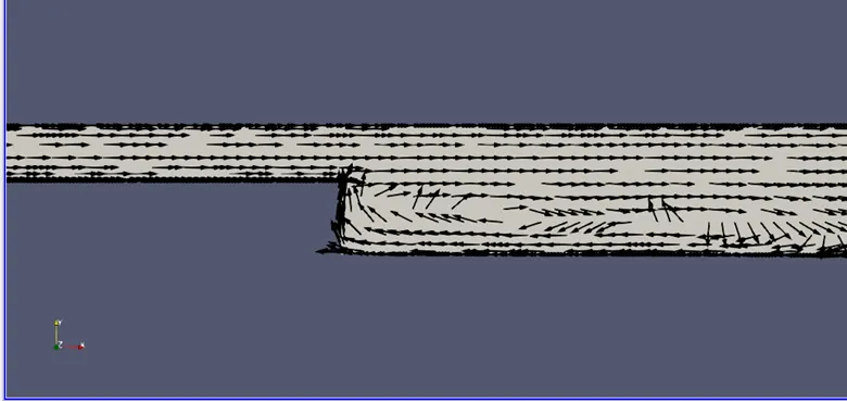
Velocity vector near recirculation
Video link:https://www.youtube.com/watch?v=V4JcR-asvLE
Case 2 : dx = 1.5e-3m, dy = 1.5e-3m, dz = 1.5e-3m
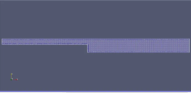
Mesh
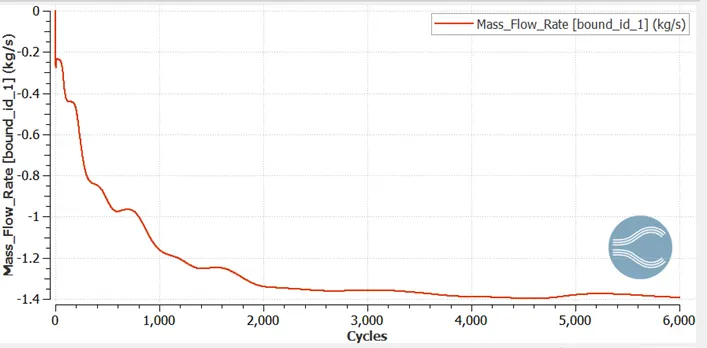
Mass flow rate
Inlet
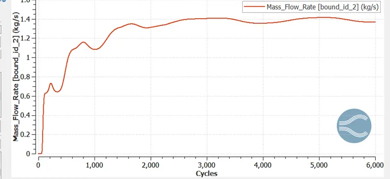
Outlet
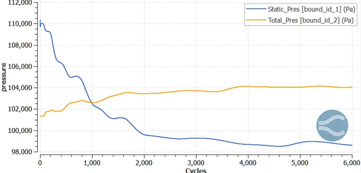
Pressure plot
Inlet and Outlet
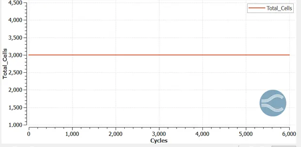
Total cells
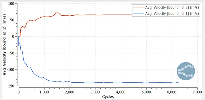
Velocity plot
Inlet and Outlet
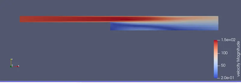
Velocity contour
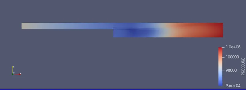
Pressure contour
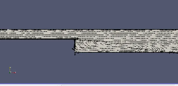
Velocity vector near recirculation
Video link:https://www.youtube.com/watch?v=fgw48hD6GYI
Case 3 : dx = 1e-3m, dy = 1e-3m, dz = 1e-3m
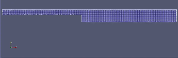
Mesh
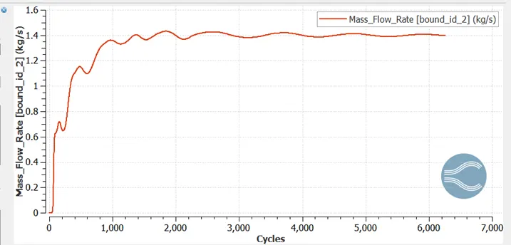
Mass flow rate
Inlet
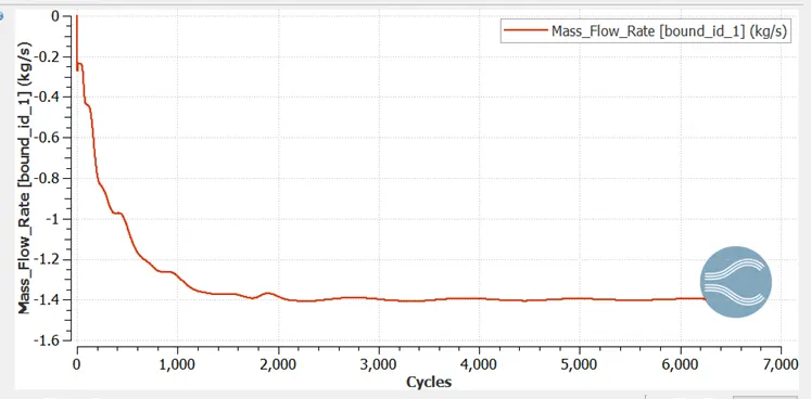
Outlet
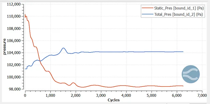
Pressure plot
Inlet And Outlet
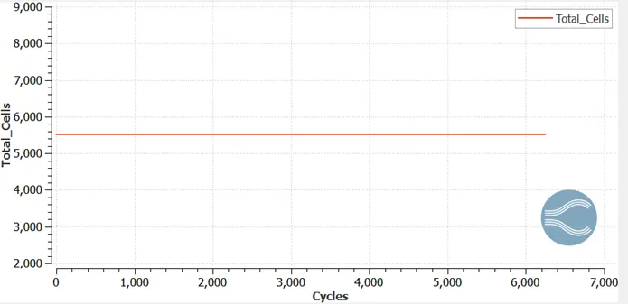
Total cells
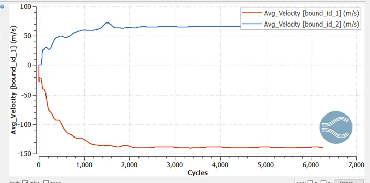
Velocity plot
Inlet and Outlet
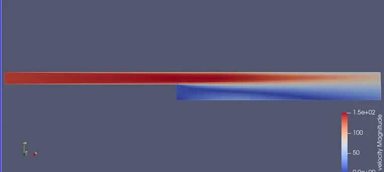
Velocity contour
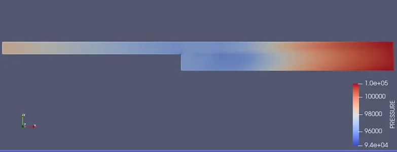
Pressure contour
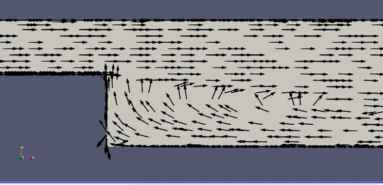
Velocity vector near recirculation
Video link:https://www.youtube.com/watch?v=n5mgT32IZpI
Flow separation:
- This is taking place at the back of the step where area is increased
- Due to positive pressure gradient created at this zone, the flow start moving backward
- As a result, the flow separates and a recirculation region is formed due to flow in opposite direction. This is also called Wake Region
Conclusion:
- Three simulations were run with different grid size and gives a necessary plots and contour
- With decrease in grid size means finer mesh the contours became smoother and more accurate results were found
- Fixed embedding gives finer mesh near the wall boundaries and its help for capturing physics nears the wall