Week 3: Flow over a backward facing step

Aim:

(i) To carry out the flow over backward facing step simulation for three different meshes.

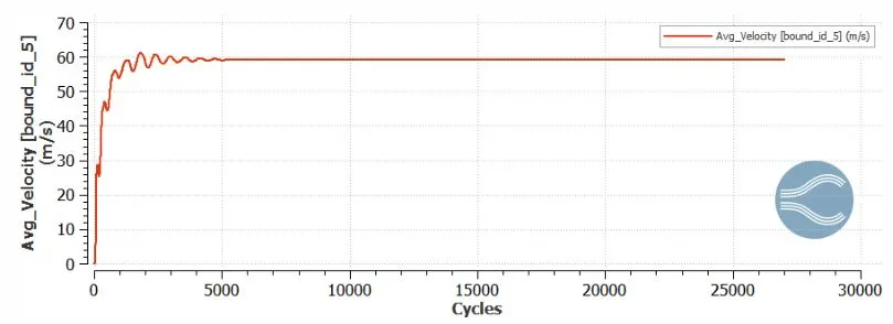
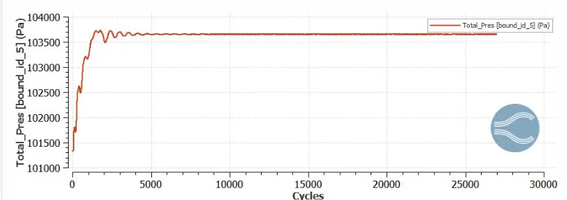
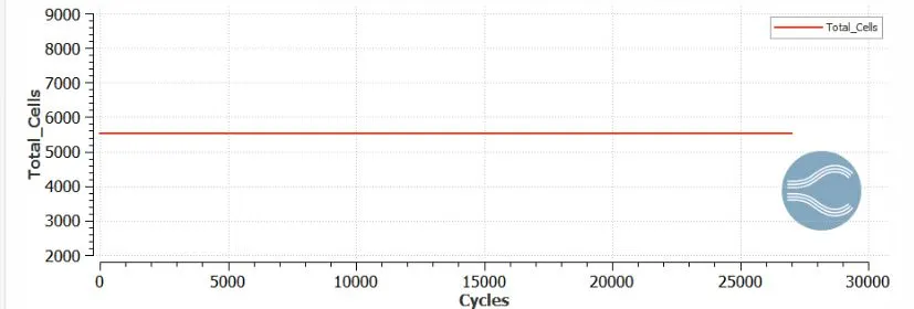
(ii) To visualize the plots of velocity, pressure, mass flow rate, total cell counts and pressure, temperature contours

(iii)To study about the flow separation

Introduction:

Backward-Facing Step flow is one representative separation flow model, which is of significance in both theoretical and engineering development. Various applications for Backward-Facing Step flow can be found in our daily life, such as the air foils at large attack angle, the spoiler flows, separation flow behind a vehicle, inlet tunnel flow of engine or inside a condenser/combustor, and also the flow around a boat or a building. It is a basic model that involves the most important features of a separated flow: free shear flow separation, vortex evolution and re-attachment. It is well known that the flow separation near the Backward-Facing Step will possibly lead to additional flow resistance and noise, and under critical conditions even for stalling of an aircraft, the general understanding of the physics in Backward-Facing Step flow has become one hot topic .As a typical kind of separation flow model , Backward-Facing Step has been studied as an important flow dynamic model for more than half a century, while the real step flow situations/ designs can be found with the early years of natural world. For an extensive period, research on the flow of channels with reversals have transformed from symmetry to asymmetry which has received great enthusiasm. To aid further numerical and experimental research on such flows, the flow through an abrupt enlargement has been regarded as a benchmark since it comprises a layout possessing among the most primary geometries. Researchers begun to generalize the basic trends in Backward-Facing Step and with the development of numerical capacities, more computational studies were published.

Theory:

Liquid or gas flow through pipes or ducts is commonly used in heating and cooling applications and fluid distribution networks. The fluid in such applications is usually forced to flow by a fan or pump through a flow section. We pay particular attention to friction, which is directly related to the pressure drop and head loss during flow through pipes and ducts. The pressure drop is then used to determine the pumping power requirement. A typical piping system involves pipes of different diameters connected to each other by various fittings or elbows to route the fluid, valves to control the flow rate, and pumps to pressurize the fluid. You have probably noticed that most fluids, especially liquids, are transported in circular pipes. This is because pipes with a circular cross section can withstand large pressure differences between the inside and the outside without undergoing significant distortion. Noncircular pipes are usually used in applications such as the heating and cooling systems of buildings where the pressure difference is relatively small, the manufacturing and installation costs are lower, and the available space is limited for ductwork. Although the theory of fluid flow is reasonably well understood, theoretical solutions are obtained only for a few simple cases such as fully developed laminar flow in a circular pipe. Consider a fluid entering a circular pipe at a uniform velocity. Because of the no-slip condition, the fluid particles in the layer in contact with the wall of the pipe come to a complete stop. This layer also causes the fluid particles in the adjacent layers to slow down gradually as a result of friction. To make up for this velocity reduction, the velocity of the fluid at the midsection of the pipe has to increase to keep the mass flow rate through the pipe constant. As a result, a velocity gradient develops along the pipe. The region of the flow in which the effects of the viscous shearing forces caused by fluid viscosity are felt is called the velocity boundary layer or just the boundary layer. The hypothetical boundary surface divides the flow in a pipe into two regions: the boundary layer region, in which the viscous effects and the velocity changes are significant, and the irrotational (core) flow region, in which the frictional effects are negligible and the velocity remains essentially constant in the radial direction. The region from the pipe inlet to the point at which the velocity profile is fully developed (Velocity gradient doesnot change in flow direction) is called the hydrodynamic entrance region, the length of this region is called the hydrodynamic entry length Lh. The velocity profile in the fully developed region is parabolic in laminar flow and much flatter (or fuller) in turbulent flow. The steady, laminar, incompressible flow of fluid with constant properties in the fully developed region of a straight circular pipe. The average velocity in fully developed laminar pipe flow is one half of the maximum velocity. Hagen– Poiseuille flow in honor of the works of G. Hagen (1797–1884) and J. Poiseuille (1799–1869) that for a specified flow rate, the pressure drops and thus the required pumping power is proportional to the length of the pipe and the viscosity of the fluid, but it is inversely proportional to the fourth power of the radius of the pipe. The average velocity in heating and cooling applications may change somewhat because of changes in density with temperature. Also, the friction between the fluid particles in a pipe does cause a slight rise in fluid temperature as a result of the mechanical energy being converted to sensible thermal energy. But this temperature rise due to frictional heating is usually too small to warrant any consideration in calculations and thus is disregarded. The flow regime in the first case is said to be laminar, characterized by Smooth streamlines and highly ordered motion, and turbulent in the second case, where it is characterized by velocity fluctuations and highly disordered motion. The transition from laminar to turbulent flow does not occur suddenly; rather, it occurs over some region in which the flow fluctuates between laminar and turbulent flows before it becomes fully turbulent. Osborne Reynolds discovered that the flow regime depends mainly on the ratio of inertial forces to viscous forces in the fluid

where = average flow velocity (m/s), = characteristic length of the geometry (diameter in this case, in m), and 𝜈 = 𝜇/𝜌 = kinematic viscosity of the fluid (m2/s). Note that the Reynolds number is a dimensionless quantity. The transition from laminar to turbulent flow depends on the geometry, surface roughness, flow velocity, surface temperature, and type of fluid, among other things.

Gravity has no effect on flow in horizontal pipes, but it has a significant effect on both the velocity and the flow rate in uphill or downhill pipes.

Turbulent flow is characterized by disorderly and rapid fluctuations of swirling regions of fluid, called eddies, throughout the flow. In turbulent flow, the swirling eddies transport mass, momentum, and energy to other regions of flow much more rapidly than molecular diffusion, greatly enhancing mass, momentum, and heat transfer. As a result, turbulent flow is associated with much higher values of friction, heat transfer, and mass transfer coefficients. The eddy motion in turbulent flow causes significant fluctuations in the values of velocity, temperature, pressure, and even density. Instantaneous velocity (or) temperature (or) Pressure is sum of averaged value of parameter and fluctuating component of parameter. The chaotic fluctuations of fluid particles play a dominant role in pressure drop, and these random motions must be considered in analyses together with the average velocity. the turbulent shear stress as consisting of two parts: the laminar component, which accounts for the friction between layers in the flow direction (expressed as 𝜏lam = −𝜇 du/dr), and the turbulent component, which accounts for the friction between the fluctuating fluid particles and the fluid body (denoted as 𝜏turb and is related to the fluctuation components of velocity). Many semi-empirical formulations have been developed that model the Reynolds stress (or) Turbulent stresses in terms of average velocity gradients in order to provide mathematical closure to the equations of motion. Such models are called turbulence models. in the early 1900s, the German engineer L. Prandtl introduced the concept of y Laminar flow y ∂u ∂y y=0 mixing length lm, which is related to the average size of the eddies that are

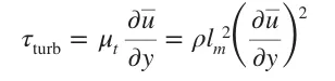
Therefore, the velocity profile is very slowly changing in the core region of a turbulent boundary layer, but very steep in the thin layer adjacent to the wall, resulting in large velocity gradients at the wall surface. So it is no surprise that the wall shear stress much larger in the turbulent flow than in laminar flow. Turbulent flow along a wall can be considered to consist of four regions, characterized by the distance from the wall . The very thin layer next to the wall where viscous effects are dominant is the viscous (or laminar or linear or wall) sublayer. The velocity profile in this layer is very nearly linear, and the flow is streamlined. Next to the viscous sublayer is the buffer layer, in which turbulent effects are becoming significant, but the flow is still dominated by viscous effects. Above the buffer layer is the overlap (or transition) layer, also called the inertial sublayer, in which the turbulent effects are much more significant, but still not dominant.

Above that is the outer (or turbulent) layer in the remaining part of the flow in which turbulent effects dominate over molecular diffusion (viscous) effects.

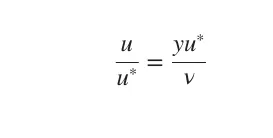
This below equation is known as the law of the wall

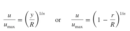
Velocity profile using power law

The friction factor in fully developed turbulent pipe flow depends on the Reynolds number and the relative roughness 𝜀 /D, which is moody chart. It is developed for circular pipes, it can also be used for noncircular pipes by replacing diameter with hydraulic diameter. But it should be kept in mind that these values are for new pipes, and the relative roughness of pipes may increase with use as a result of corrosion, scale buildup, and precipitation. As a result friction factor may increase by a factor 5-10.

The fluid in a typical piping system passes through various fittings, valves, bends, elbows, tees, inlets, exits, expansions, and contractions in addition to the straight sections of piping. These components interrupt the smooth flow of the fluid and cause additional losses because of the flow separation and mixing they induce. In a typical system with long pipes, these losses are minor compared to the head loss () in the straight sections (the major losses) and are called minor losses. Loss coefficient () is given by

however, it is based on the additional irreversible loss of mechanical energy that would otherwise not exist if the minor loss component were not there. The loss coefficient, in general, depends on the geometry of the component and the Reynolds number.

minor losses are also expressed interms of equivalent length ()

represents as friction factor

Minor losses due to geometry shapes are

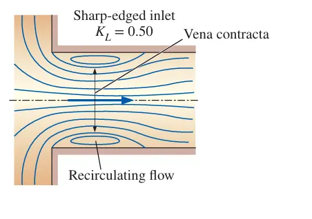
a. The head loss at the inlet of a pipe is a strong function of geometry. It is almost negligible for well-rounded inlets (KL = 0.03 for r/D > 0.2), but increases to about 0.50 for sharp-edged inlets . That is, a sharp-edged inlet causes half of the velocity head to be lost as the fluid enters the pipe. This is because the fluid cannot make sharp 90° turns easily, especially at high velocities. As a result, the flow separates at the corners, and the flow is constricted into the vena contracta region formed in the midsection of the pipe. Therefore, a sharp-edged inlet acts like a flow constriction. The velocity increases in the vena contracta region (and the pressure decreases) because of the reduced effective flow area and then decreases as the flow fills the entire cross section of the pipe. There would be negligible loss if the pressure were increased in accordance with Bernoulli’s equation (the velocity head would simply be converted into pressure head). However, this deceleration process is far from ideal and the viscous dissipation caused by intense mixing and the turbulent eddies converts part of the kinetic energy into frictional heating, as evidenced by a slight rise in fluid temperature. The end result is a drop in velocity without much pressure recovery, and the inlet loss is a measure of this irreversible pressure drop.

b. Piping systems often involve sudden or gradual expansion or contraction sections to accommodate changes in flow rates or properties such as density and velocity. The losses are usually much greater in the case of sudden expansion and contraction (or wide-angle expansion) because of flow separation. By combining the equations of mass, momentum, and energy balance, the loss coefficient for the case of a sudden expansion is approximated as

. No such relation exists for a sudden contraction, and the KL values in that case must be read from a chart or table. The losses due to expansions and contractions can be reduced significantly by installing conical gradual area changes between small and large pipes. velocity in the small pipe is to be used as the reference velocity . Losses during expansion are usually much higher than , losses doing contraction because of flow separation. Piping systems also involve changes in direction without a change in diameter, and such flow sections are called bends or elbows. The losses in these devices are due to flow separation on the inner side and swirling secondary flow

Valves are commonly used in piping systems to control flow rates by simply altering the head loss until the desired flow rate is achieved. For valves it is desirable to have a very low loss coefficient when they are fully open, such as with a ball valve, so that they cause minimal head loss during full load operation

Case setup:

1.Started by selecting the new project on the Converge_Studio_3.1

Geometry Creation

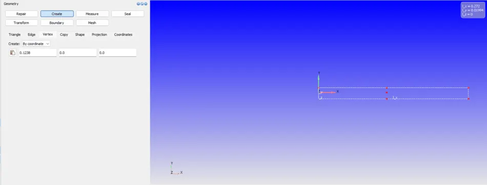
2.Geometry->create->vertex->inputs->apply. With this ,created a 7 vertices of Planar backward geometry

Vertices are (0,0,0),(0,0.0085,0),(0.1238,0.0085,0),(0.272,0.0085,0),(0.272,-0.0114,0),(0.1238,-0.0114,0),(0.1238,0,0).

3.Geometry->create->triangles->from three points. Select the three vertices and then apply.

To create the plane of the geometry then need to repeat the above step for four more times.

4.Geometry->create->copy. Selecting the Boundary then giving an offset inputs and then apply.

This will copy and offset the created surface

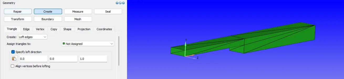
5.Geometry->create->Triangle->loft edges. Selecting the planar surfaces and then apply.

This will join the planar surfaces and creates a volume

Aligning normal

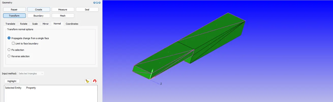
6.Geometry->Transform->Normal and propagate change from single face and select the boundary and then click apply.

This will align the normal towards region, Fluid flowing.

Boundary Flagging

7.Geometry->Boundary->Flag->create a new boundary. check the create multiple Boundaries and specify the required no of boundaries and click ok

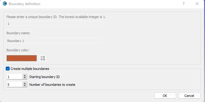
created a 5 boundaries

8.Selecting the geometry Boundaries and then select boundary flags and click apply and rename the flags

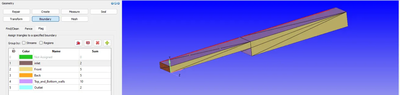
Assigning the boundary to the flags

9.Diagnosis tab and click on find. Message appeared is shown below

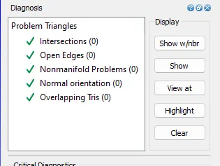
This step is carried out to find the problems present in the geometry. Above message shows there is no problems present in the geometry

Assigning the application type of flow

10.Begin case setup option is clicked. Application Type is selected as time-based

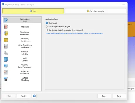
Time-based application type utilized for both steady state and transient flow.

Assigning a materials and its properties

11.Selecting the materials then check both gas and species and air is mentioned for pre-defined mixtures.

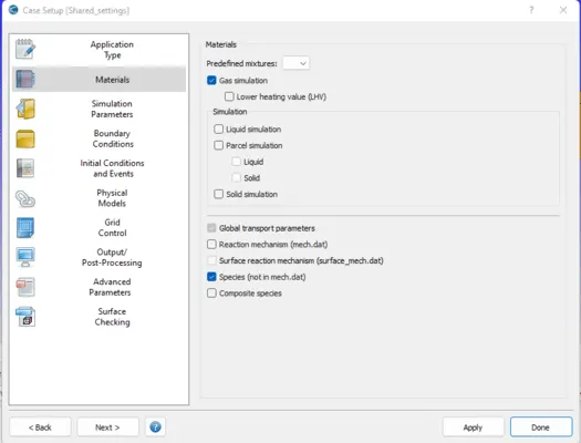
working fluid is air, basically air is gas that is the reason for selecting gas simulation. Air is composed based on different species present in nature. Species also included.

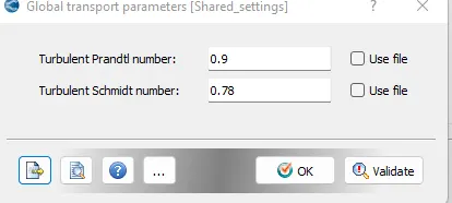
12.Global Transport parameters is selected and click ok.

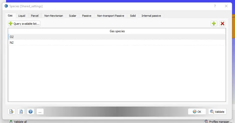
13.species is selected then clicking an add symbol then N2 and O2 is selected and click Ok.

Assigning a type of flow

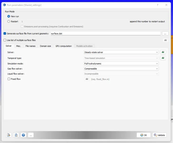
14.Steady state solver utilizing this type of application and the flow is characterized as compressible and choose the momentum and energy equations to solve.

Assigning a time parameters

15.selecting the simulation time parameters allow to input the maximum no of iterations, minimum timestep, maximum timestep, etc...,

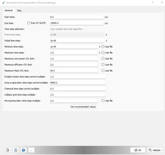
Choosing the solver

16.Selected the solver parameters to choose the pressure-velocity coupling algorithm, Navier-stokes Equation. Specifying the tolerance, max, min no of iterations for the solver, choosing the numerical schemes etc...,

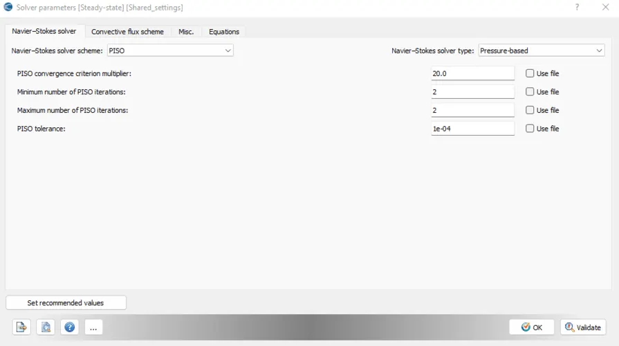
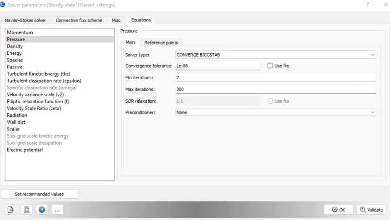
Describing the regions

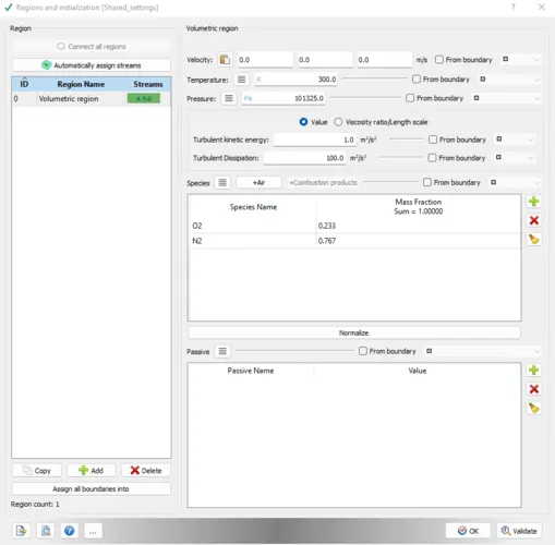
17.Region is described with initial conditions. Regions and initialization is selected, created the region and given the inputs for the initialization.

Assigning the conditions to the boundary

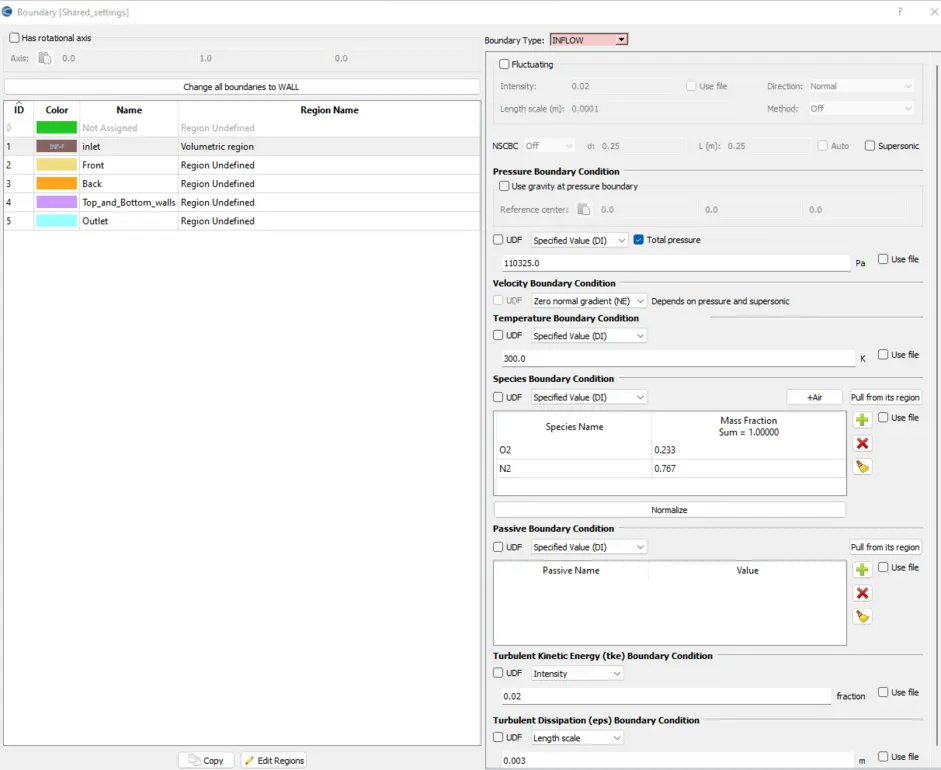
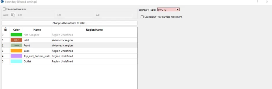
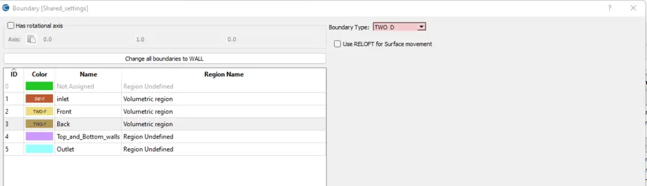
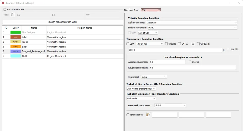
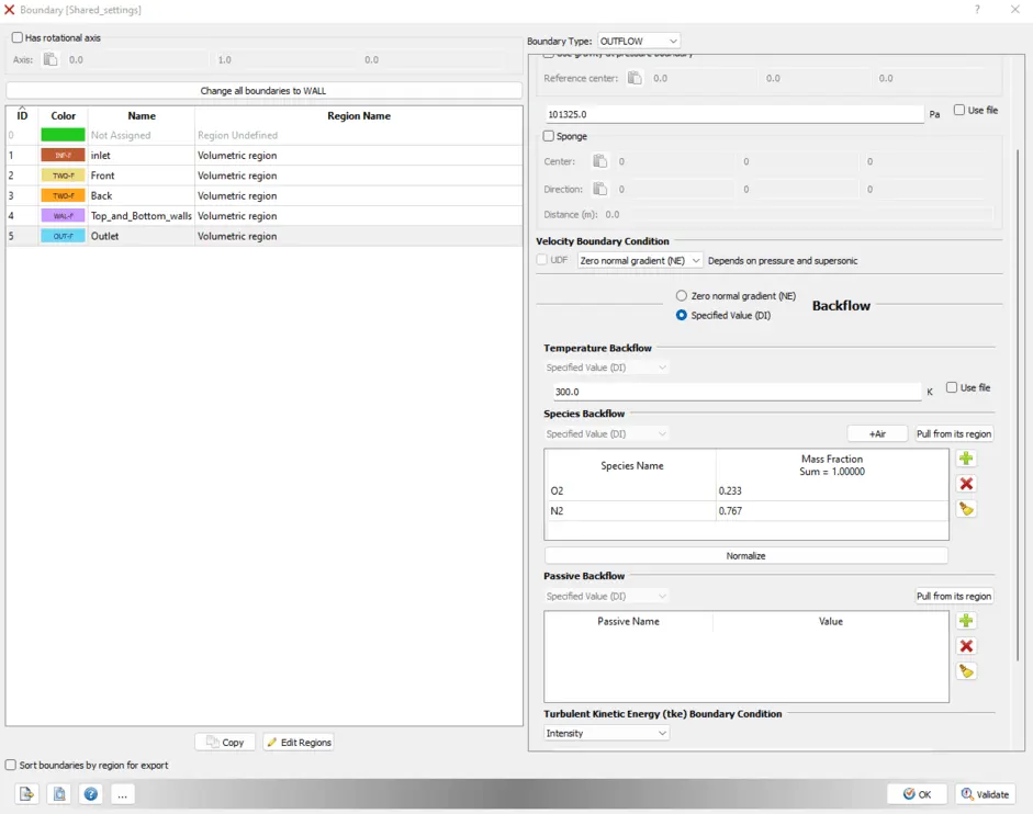
18.selecting the boundary and assigning the conditions to the boundary flagging's

Creating the monitor plots

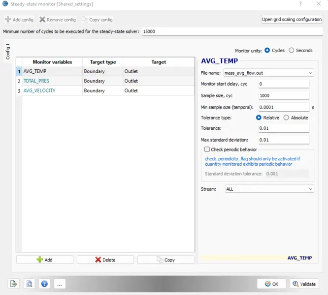
19.selecting the steady state monitor and add config and provide the input for minimum no of cycles to run and add the monitor variables of the boundary at outlet and add sample size in terms of cycles.

setting up the physics

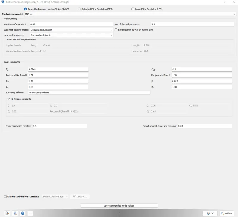
20. Selecting the physics modelling and check the turbulence modelling

select the turbulence modeling from case setup and chosen the k- RNG turbulence model.

Mesh settings for the domain

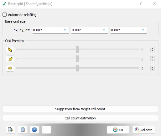
21. Selecting the base grid and given the input of mesh length in each direction

22. Selecting the grid control will allows to include features called Adaptive Mesh Refinement, fixed embedding

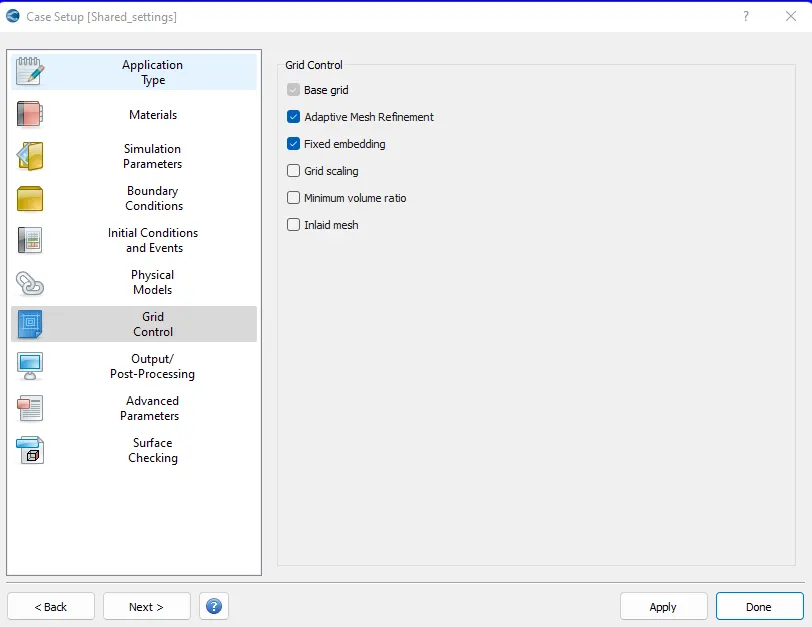
23.Selecting the fixed embedding and given inputs as boundary and boundary is selected as top and bottom walls and scale to 1.

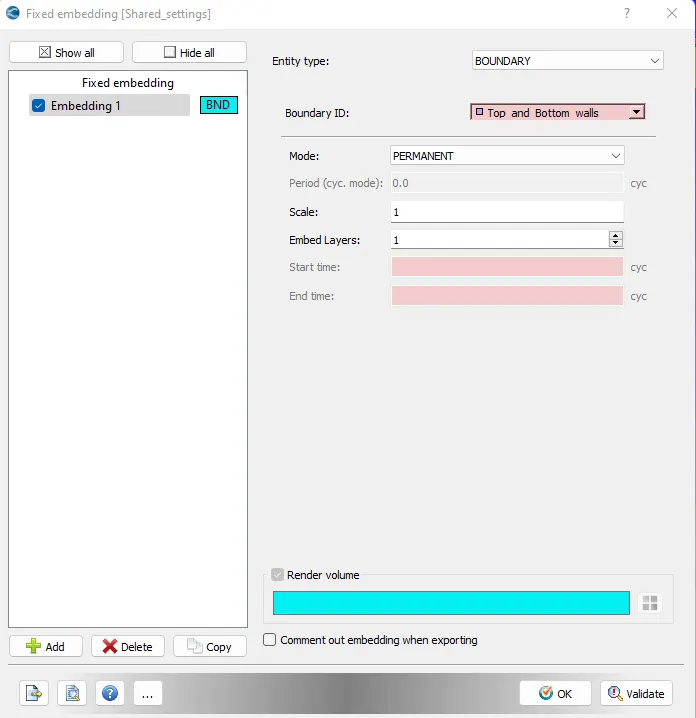
This will create a layer of fine mesh near the walls

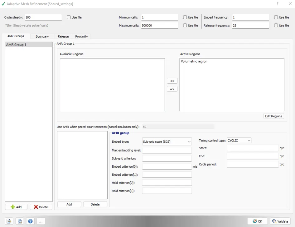
24.Selecting the adaptive mesh refinement and providing input as maximum cells as 5,00,000 and selecting the volumetric region

output files Setup:

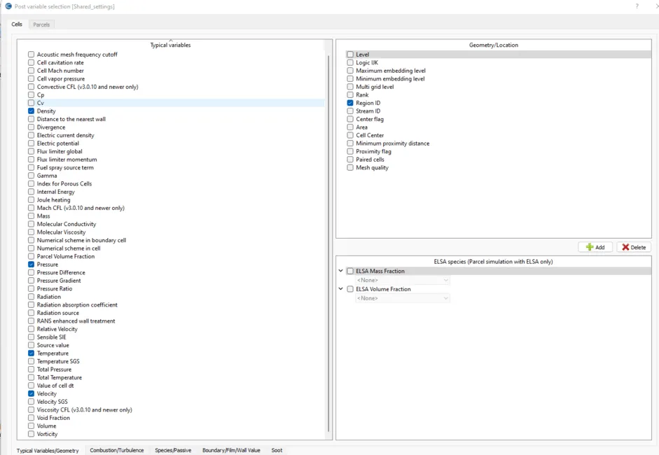
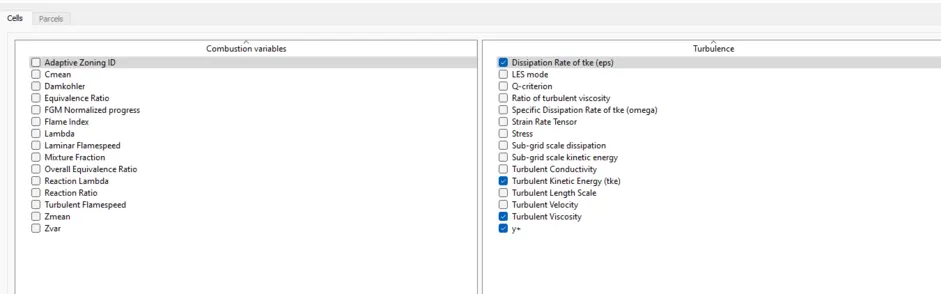
25.Post variable selection is selected from case setup, then selecting the typical flow variable, turbulence variables.

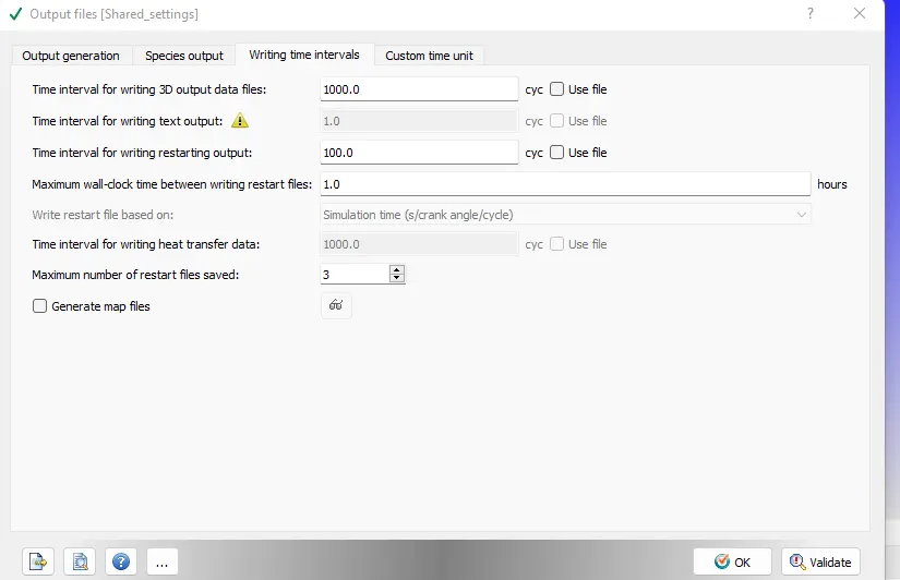
26.selecting the output files and given input in cycles to write output files, restart files etc

after exporting the files using export option and then open the cygwin terminal ,navigate the folder and enter the command to run the simulation.

Mesh:

BaseMesh:

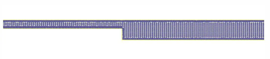
Medium size Mesh:

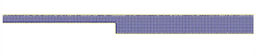
Fine Size Mesh:

Plot:

Base Mesh:

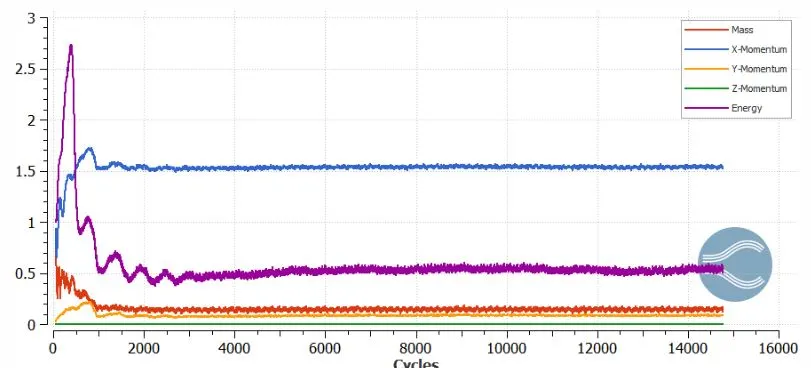
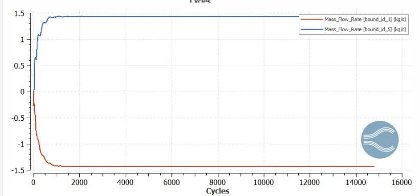
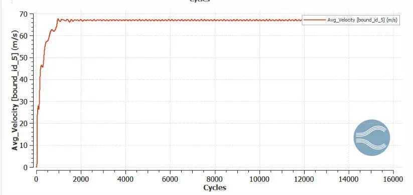
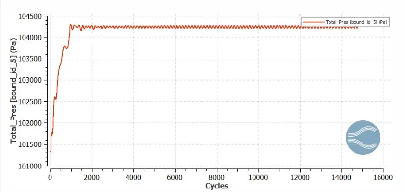
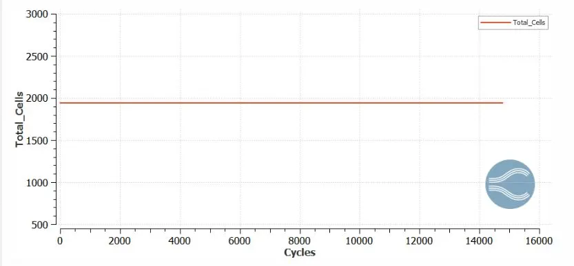
Medium Mesh

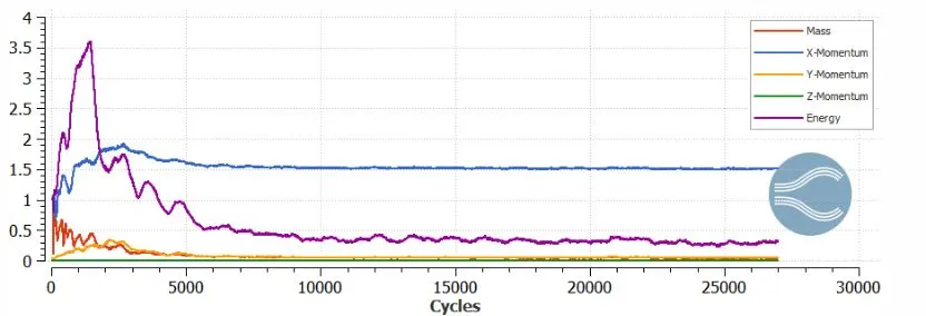
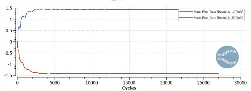
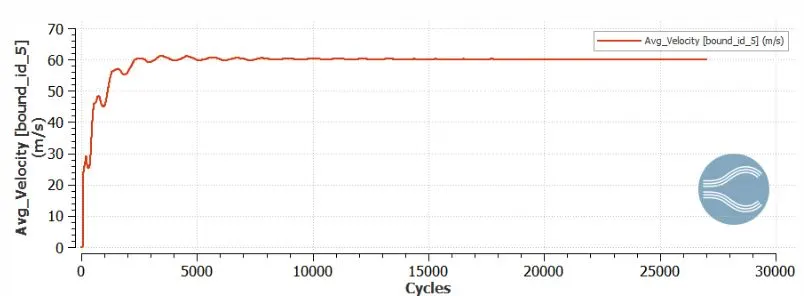
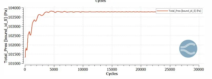
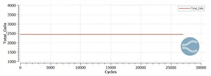
Fine Mesh:

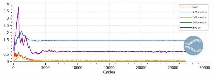
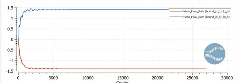
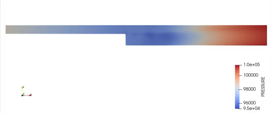
Pressure Contour:

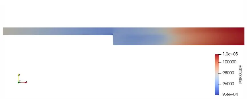
Base Mesh:

Medium size mesh:

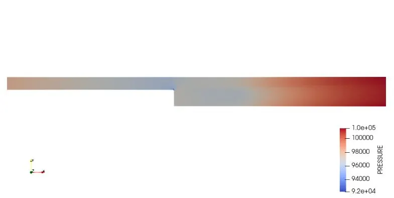
Fine Mesh:

Velocity Contour

Base Mesh

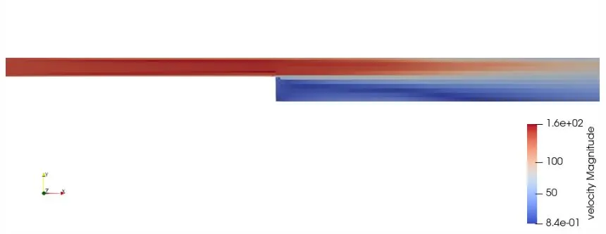
Medium size mesh:

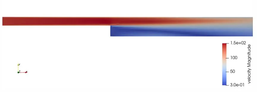
Fine Mesh:

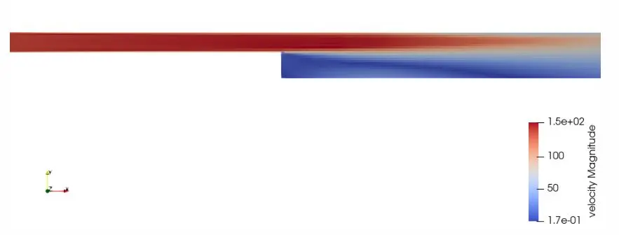
Velocity Vector

Base Mesh

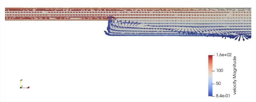
Medium size mesh:

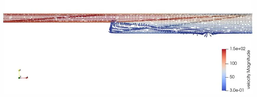
Fine Mesh:

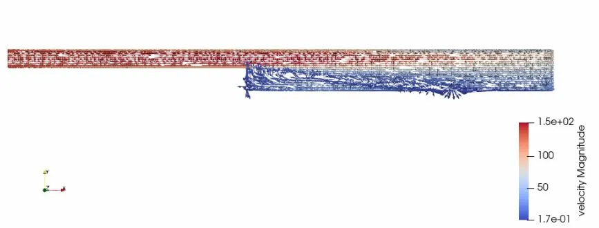
Conclusion:

1.Flow over the backward facing step simulations is executed on converge CFD with three mesh sizes.

2.Static pressure decreases from the inlet to the backward facing step.Due to sudden expansion the static pressure will drop. From there the static pressure increases due to increases in area.

3.Flow separation occurs when the sudden expansion takes place on the pipe due to pressure drop. velocity increases, Velocity increased flow will travel without changing the direction. Due to this circulation region forms on the low-pressure region.

4.Velocity is increased after the backward step we can observe the drop in the velocity.