Flow over a backward facing step

Flow over a backward facing step

• Aim:

- Simulate air flow inside a backward facing step

- Perform grid independence by refining the mesh size

- Post processing the required physical parameters

• Theory:

1. Backward facing step flow:

Many industrial application involves flow separation and reattachment. To illustrate the above phenomenon, flow simulation over backward facing step is considered. Flow through a backward facing step is one of the classical internal flow problem in fluid mechanics. Extensive numerical and experimental studies have been done on this issue. Due to the geometric simplicity and flow diagnostic technique, this phenomena has become a practice for numeric validation for computational fluid dynamics (CFD).

2. Flow separation:

Flow separation or boundary layer separation is the detachment of a boundary layer from a surface into a wake. Separation occurs in flow that is slowing down, with pressure increasing, after passing the thickest part of a streamline body or passing through a widening passage. Flowing against an increasing pressure is known as flowing in an adverse pressure gradient. The boundary layer separates when it has travelled far enough in an adverse pressure gradient that the speed of the boundary layer relative to the surface has stopped and reversed direction. The flow becomes detached from the surface, and instead takes the forms of eddies and vortices. The fluid exerts a constant pressure on the surface once it has separated instead of a continually increasing pressure if still attached.

3. Adverse pressure gradient:

In fluid dynamics, an adverse pressure gradient occurs when the static pressure increases in the direction of the flow. This is important for boundary layers. Increasing the fluid pressure is akin to increasing the potential energy of the fluid, leading to a reduced kinetic energy and a deceleration of the fluid. Since the fluid in the inner part of the boundary layer is slower, it is more greatly affected by the increasing pressure gradient. For a large enough pressure increase, this fluid may slow to zero velocity or even become reversed causing a flow separation. This has very significant consequences in aerodynamics since flow separation significantly modifies the pressure distribution along the surface and hence the lift and drag characteristics.

• Procedure:

1. Upload the stl file onto converge studio, Perform diagnosis to check for any geometry errors.

2. Change the scale to meters if the geometry is in terms of meters by going to scale option under transform.

3. Invert the normals of each triangles to inside of the wall since we are dealing with internal flows.

4. Assign boundaries for the backward facing step. Inlet, outlet, top and bottom wall and front and back 2D walls.

- Case setup:

1. Application type: time based

2. Materials:

a. Gas simulation: air

b. Global transport properties: Deafult

c. Species: O2 and N2

3. Simulation parameters:

a. Run parameters:

Steady state solver, full hydrodynamic, compressible

Steady state mointor turned ON:

i. Average velocity

ii. Total pressure

iii. Mass flow rate

b. Simulation time parameters:

- End time- 15000 cycles

- Time step- 1e-6

- min time step- 1e-6

- max time step- 1

- Convection CFL number- 0.5

c. Solver Parameters [Steady-State]-

- Solver type- density based solver

- Equations- pressure- change preconditioner to none

- steady state solver control- convection CFL limit- 0.5

4. Boundary Conditions-

a. Inlet- Inflow

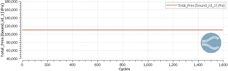
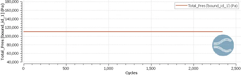
- Total pressure- 110325 Pa

- Initial temp- 300K

- Species boundary condition- add air

b. Outlet- Outflow

- Pressure- 101325 Pa

- Backflow - temp= 300k

- add air

c. Top-bottom-walls- Walls

no slip condition- The contact region between wall surface and fluid region tends to create high friction and create a 0 velocity of fluid flow, and due to viscosity of fluid, the fluid layers tend to undergo shear stress and have high pressure and overlap on eachother which eventually forms a fully developed region where velocity is max and constant and having low pressure.

d. Front and back wall: 2D- Since we are dealing with a 2D simulation the front and back regions can be considered as a symmetry or 2D wall condition.

5. Initial Conditions and Events:-

- Regions and Initialization:

Add air and Change the mass fraction of O2 to 0.77 and N2 to 0.23 so that we can notice the changes while post-processing and also even if the composition is different from the actual mole fractions of air, Converge still accepts the inputs and gives results according to its input. Therefore it can understand that the simulation takes place as long the case setup is correct and mole fraction sums up to 1.

6. Physical Models:-

- K-w SST

7. Grid Control:-

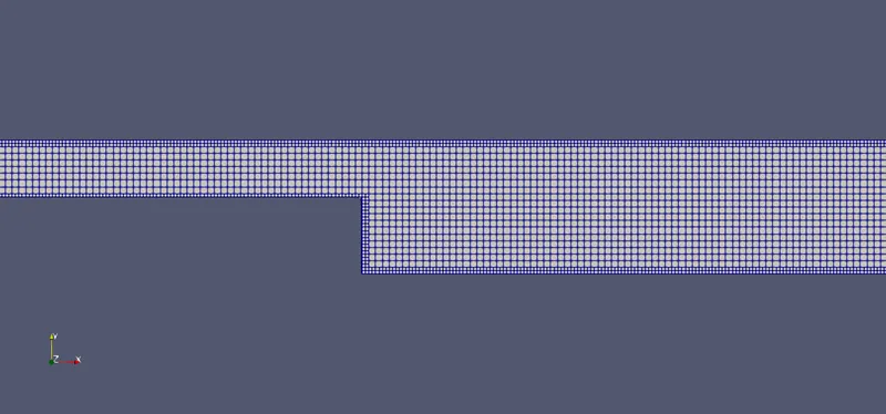
a. Base Grid:

case-1, dx = 2e-4m, dy = 2e-4m, dz = 2e-4m

case-2, dx = 1.5e-4m, dy = 1.5e-4m, dz = 1.5e-4m

case-3, dx = 1.0e-4m, dy = 1.0e-4m, dz = 1.0e-4m

b. Embedding:

- Boundary type, Near the top and bottom walls entity type, permanent mode embedding.

Embedding is the means by which we can refine the mesh to a value that is lower than the prevalent base size. This is especially useful if we are looking to refine near wall to capture the boundary layer or the wake of a body more accurately.

8. Post-Processing:-

- Post Variable Selection:

Select the parameters needed to be post processed.

Select N2 and O2 in mole fraction under species.

- Output files:

We need to set a time interval for the files to be saved during each set of iterations. It is best suited to have a min of 100 saved files for every simulation. Therefore we need to calculate the time interval for writing the output files based on our end time given in run parameters.

Restart files help in restoring the files if there is a sudden power cut/ crash which is not helpful or might end up loosing the entire data, therefore the restart files helps in resuming the simulation form the point we lost contact. Restart files time interval can be same as the writing files interval which is safe and healthy.

In this case- since the end time is 15000, we can have a time interval of 150 and the total files created will be 100.

• Results:

1. Grid size:

a. 2e-4:

- Mesh grid:

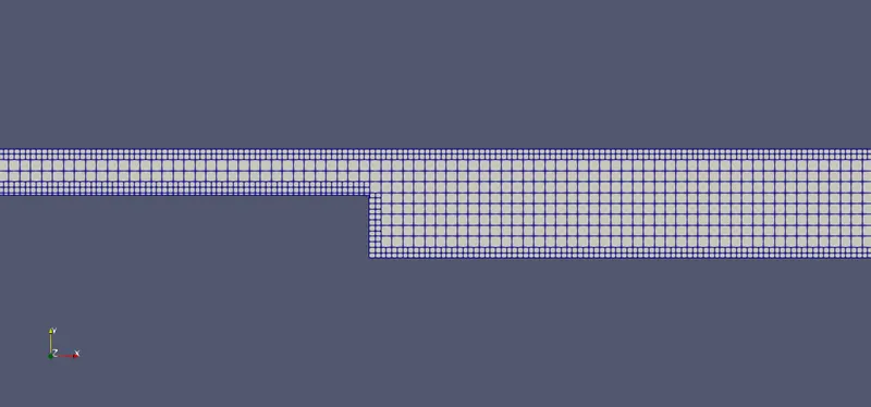
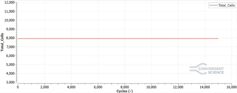
- Cell count:

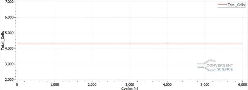
b. 1.5e-4:

- Mesh grid:

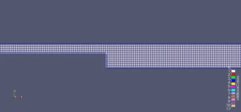
- Cell count:

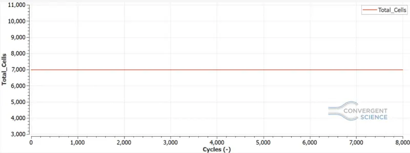
c. 1e-4:

- Mesh grid:

- Cell count:

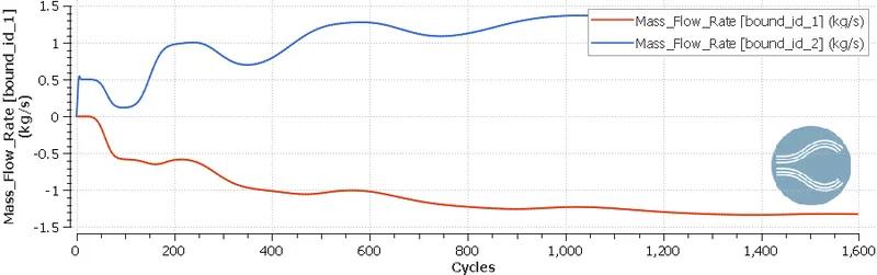
2. Outputs at grid size 2e-4:

a. Mass flow rate:

b. At inlet:

- Total pressure:

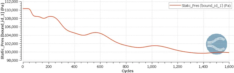
- Static pressure:

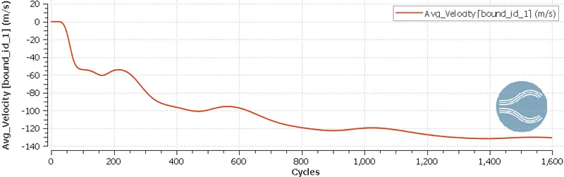
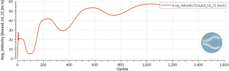
- Average velocity:

c. At outlet:

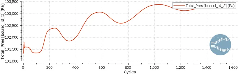
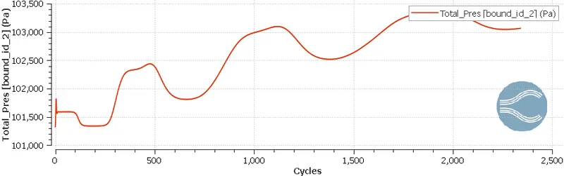
- Total pressure:

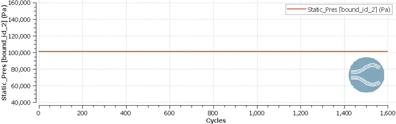
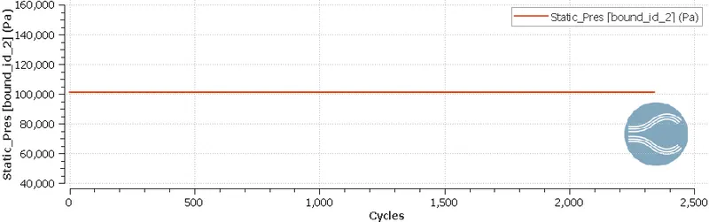
- Static pressure:

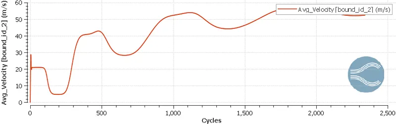
- Average velocity:

d. Velocity:

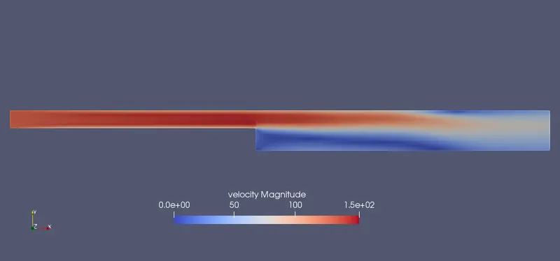
- Flow contour:

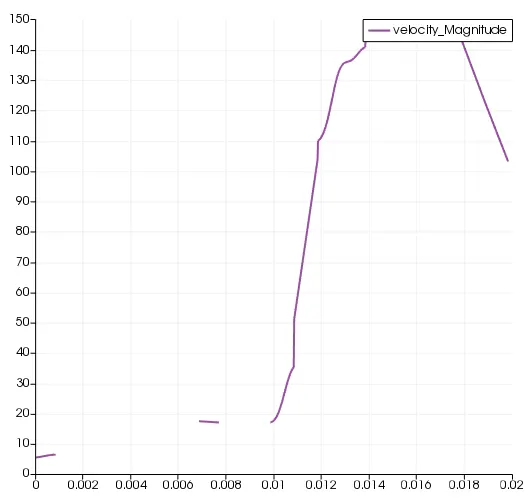
- Velocity magnitude at the separation region:

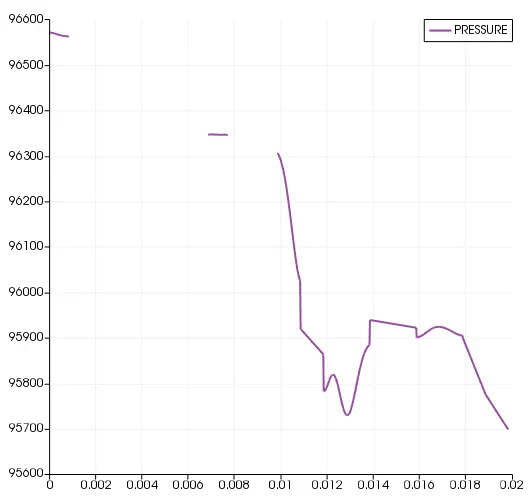
e. Pressure:

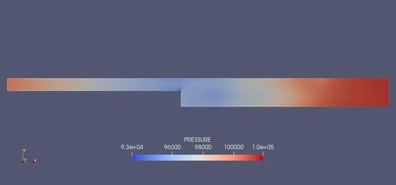
- Pressure contour:

- Pressure at the separation region:

f. Flow animation:

- Velocity:

- Pressure:

3. Outputs at grid size 1.5e-4:

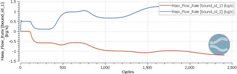
a. Mass flow rate:

b. At input:

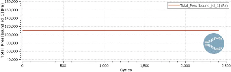
- Total pressure:

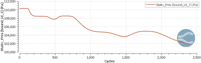
- Static pressure:

- Average velocity:

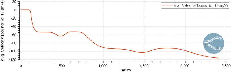
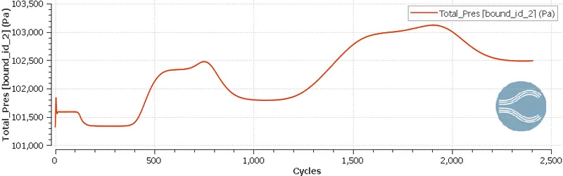
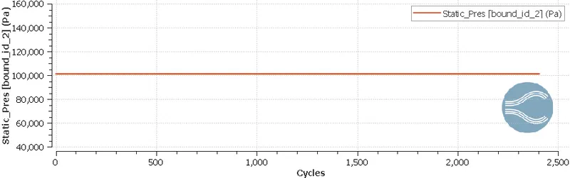
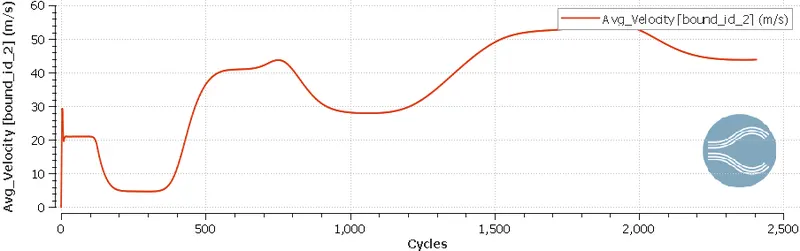
c. At outlet:

- Total pressure:

- Static pressure:

- Average velocity:

d. Velocity:

- Velocity contour:

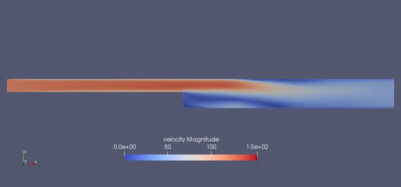
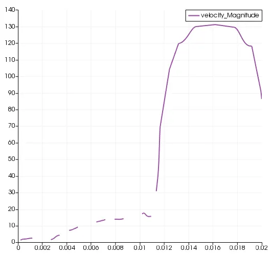
- Velocity magnitude at separation point:

e. Pressure:

- Pressure contour:

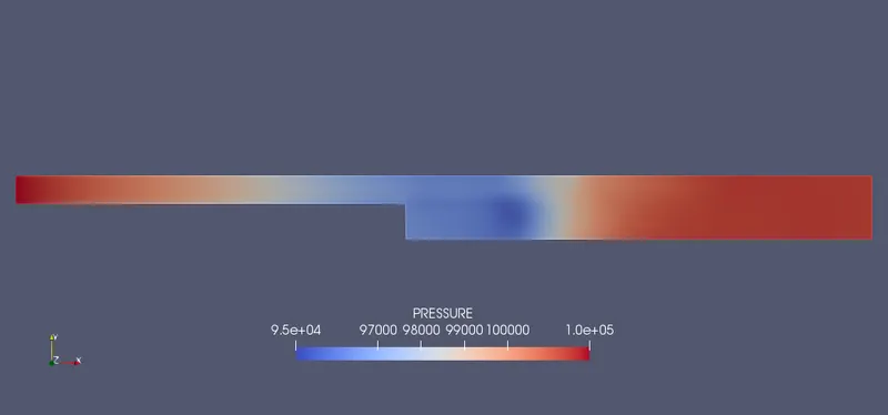
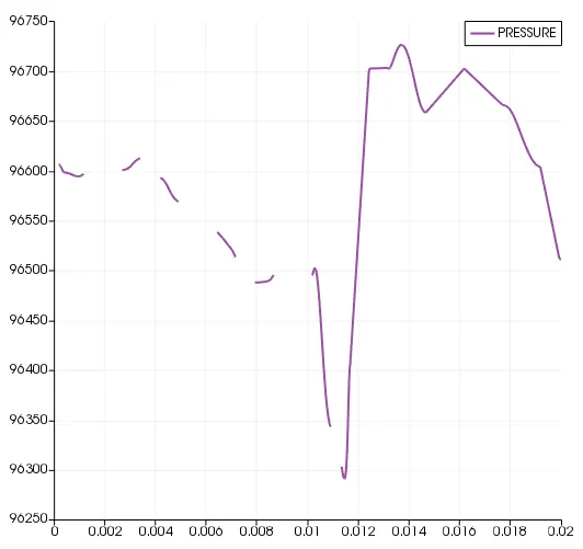
- Pressure at separation point:

f. Flow animation:

- Velocity:

- Pressure:

4. Outputs at grid size 1e-4:

a. Mass flow rate:

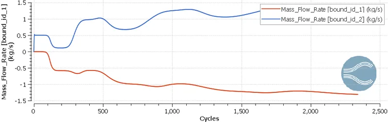
b. At inlet:

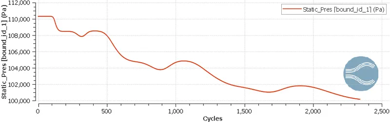
- Total pressure:

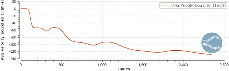
- Static pressure:

- Average velocity:

c. At outlet:

- Total pressure:

- Static pressure:

- Average velocity:

d. Velocity:

- velocity contour:

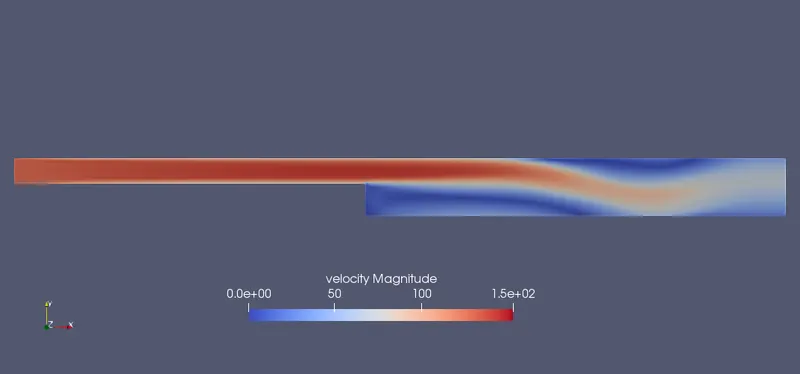
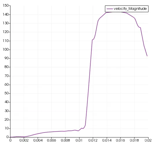
- Velocity magnitude at separation point:

e. Pressure:

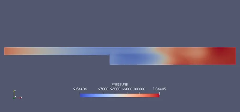
- Pressure contour:

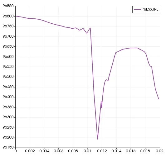
- Pressure at separation point:

f. Flow animation:

- Velocity:

- Pressure:

• Discussions:

1. Backward facing step can help in analysing the physics near the boundary level.

2. Flow separation results in 0 wall shear stress this inturn creates a pressure increaing and resulting in the opposite flow velocity and causing an adverse pressure gradient.

3. When the Pressure tends to increase after the flow separation point, potential energy develops at the local boundary layer and this causes the reduce the kinetic energy and therefore the velocity reduces.

4. Flow separation can be reduced by modifying the geometry of the object induced to flows where boundary layer is continous and separation occurs at a minimum amount.

5. Flow separation tends to reduce lift and increase static pressure, which can lead to stall for aerodynamic structures.

6. Flow separation creates a wake region at the flow end which causes a recirculation region due to the adverse pressure gradient, creating turbulence and formation of eddies.

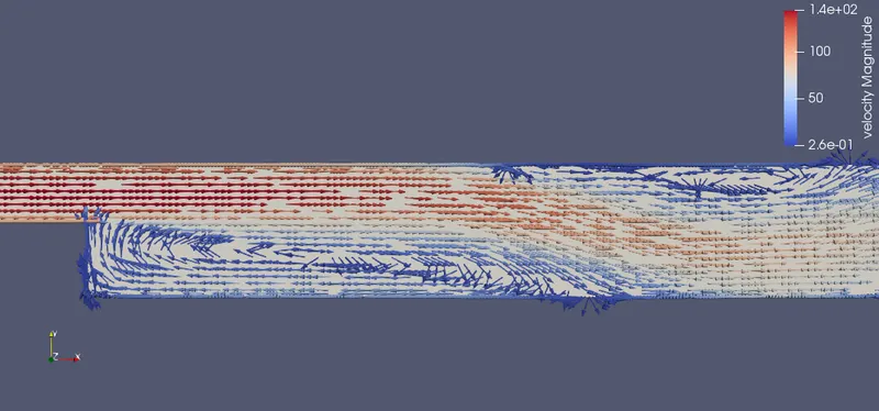
This vector image helps us in understanding the flow phsyics at the separation region where pressure gradient increases and causes recurculation region.